
When you tap a calculator app, ask a spreadsheet to total a budget, or let a navigation app choose a route, the result appears almost instantly. It is easy to think of computing as something that began with screens, keyboards, and microchips.
For centuries, however, people faced the same underlying problem: how can we perform long chains of calculation accurately, repeatably, and with less human effort? Early answers involved beads, gears, levers, punched cards, and rooms full of noisy electrical equipment.
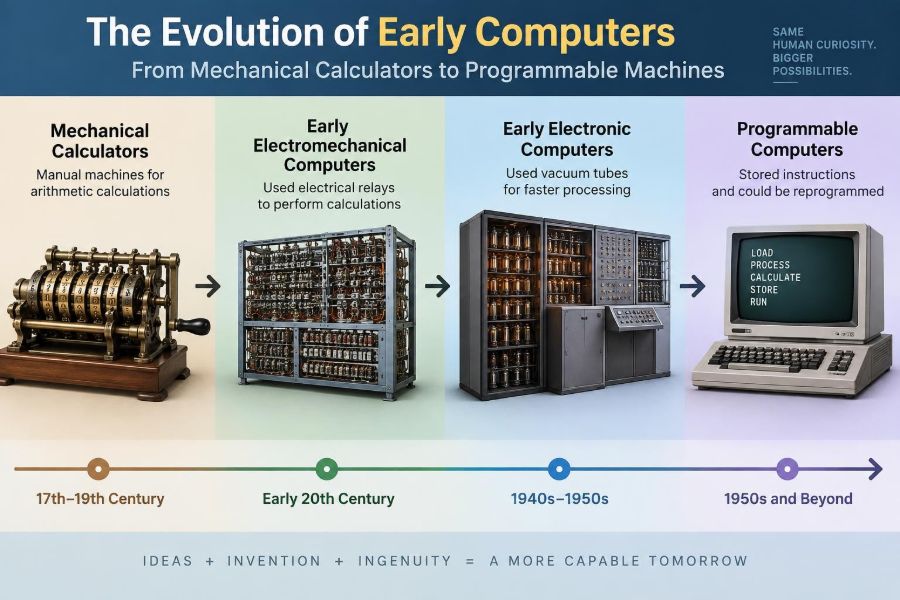
The path from a mechanical calculator to a programmable machine was not a single invention. It was a gradual shift in what machines could represent, what instructions they could follow, and how reliably they could store and process information.
Understanding that shift makes modern computing less mysterious. Many ideas behind software, memory, input, output, debugging, and automation were already taking shape long before the personal computer.
🧮 Computing Began as Organized Calculation
At its broadest, computing means carrying out a defined process to transform information into a result. The information might be numbers, names, measurements, or symbols; the process might be simple addition or a complicated scientific procedure.
Before electronic machines, a computer could mean a person whose job was to calculate tables for navigation, astronomy, engineering, or finance. Machines were built not because people could not calculate, but because manual work was slow and vulnerable to small, costly errors.
📜 The Abacus and Physical Number Representation
The abacus is one of the oldest enduring calculation tools. Beads moved along rods represent values according to their position, allowing a trained user to add, subtract, multiply, and divide efficiently.
It was not automatic: a person still decided each step. Yet the abacus introduced a lasting computing idea: represent an abstract number with a physical state. A bead’s position stands for a value, much as a modern memory cell stores a bit.
⚙️ Why Gears Changed the Possibilities
Mechanical calculators used gears, wheels, and carry mechanisms to encode decimal digits. Turning a wheel could advance another wheel after a full rotation, physically implementing the carry operation used in ordinary arithmetic.
This was significant because the mechanism, rather than the operator, enforced part of the mathematical rule. Once configured, a device could perform repeated arithmetic operations consistently. Its limitations were equally clear: precision engineering was expensive, gears wore down, and complex operations required many moving parts.
➕ Pascal’s Adding Machine
In the 1640s, Blaise Pascal designed the Pascaline, a mechanical calculator intended to help with accounting calculations. Its numbered wheels could add and subtract, using linked mechanisms to carry values between decimal places.
The Pascaline was difficult to manufacture and not a general-purpose computer. Still, it demonstrated that arithmetic could be embodied in hardware. A calculation no longer had to exist only as a sequence of human decisions on paper.
✖️ Leibniz and Repeated Operations
Gottfried Wilhelm Leibniz improved on earlier ideas with a stepped-drum mechanism. This arrangement made multiplication and division more practical by turning multiplication into repeated addition and division into repeated subtraction.
That strategy remains conceptually useful. A complex-looking task is often broken into simpler operations a machine can perform reliably. Modern processors use vastly different technology, but they also execute sophisticated programs through combinations of basic operations.
🧱 Mechanical Limits Were Real Limits
Mechanical calculators could be ingenious but fragile. Friction, imperfect parts, limited speed, and the effort of setting values constrained what they could do. Adding more features often meant adding more physical complexity.
These machines also usually lacked a way to store a long procedure. A human operator had to remember the method, manipulate controls, and record intermediate answers. Automation had begun, but it was not yet programming in the modern sense.
🧵 Jacquard Looms and Instructions in Cards
In the early nineteenth century, the Jacquard loom used punched cards to control weaving patterns. Holes and non-holes determined which threads were lifted, allowing intricate designs to be reproduced without manually directing every motion.
The loom did not calculate numbers, but it established a powerful principle: instructions can be encoded in a separate, reusable physical medium. Change the card sequence and the same machine produces a different pattern. This separation of machine from instructions is central to programmability.
🗃️ Punched Cards as Information Carriers
A punched card can represent information through the presence or absence of holes at specified positions. The exact meaning depends on the system: a position might stand for a command, a number, a letter, or a category.
Cards had practical advantages. They could be prepared in advance, copied, sorted, and inspected. They also had drawbacks: they were bulky, could be damaged or put in the wrong order, and made rapid interactive changes difficult.
🏭 Babbage’s Difference Engine
Charles Babbage designed the Difference Engine to calculate mathematical tables using the method of finite differences. This method can generate values of certain polynomial functions through repeated addition, avoiding the need to perform multiplication for every entry.
Accurate printed tables mattered greatly in navigation, engineering, and science. Errors in manually copied tables could spread into real-world decisions. Although Babbage’s full early design was not completed in his lifetime, the project showed how a specialized machine could automate a substantial calculation workflow.
🧠 The Analytical Engine’s Bigger Idea
Babbage’s later Analytical Engine was more ambitious. It was designed as a machine that could perform many different kinds of calculations, directed by punched cards rather than fixed for one mathematical task.
Its design anticipated several familiar concepts: a processing unit called the mill, storage called the store, input through cards, and output such as printed results. It was never fully built as envisioned, so it should not be described as a working modern computer. Its architectural ideas, however, were remarkably influential.
🔀 Control Flow Makes Programs Flexible
A useful program needs more than a list of arithmetic operations. It may need to repeat steps until a condition is met or choose between actions depending on a result. These are forms of control flow.
The Analytical Engine design included conditional branching and loops. A conditional branch means the next instruction depends on a value, while a loop repeats a sequence. For example, a program calculating a total might repeat “read value, add value” until no more values remain.
👩💻 Ada Lovelace and Algorithms for Machines
Ada Lovelace wrote extensive notes on the Analytical Engine, including a method for calculating Bernoulli numbers. Her work is often recognized as an early published description of an algorithm intended for a general-purpose machine.
She also saw that a machine manipulating symbols could potentially work with more than ordinary arithmetic, provided relationships were expressed in a suitable form. That was a conceptual leap: computing is not defined by numbers alone, but by rule-based transformation of represented information.
📊 Census Data Created a New Scale Problem
As governments and organizations collected more records, handling information became a major operational challenge. Counting and categorizing data by hand could take years, especially when millions of forms were involved.
Herman Hollerith developed punched-card tabulating equipment for processing census data in the late nineteenth century. Operators encoded facts on cards; machines sensed holes and counted categories. This was not general-purpose programming, but it was a major step toward automated data processing.
🔌 Tabulators Linked Input, Processing, and Output
Tabulating systems made the information pipeline visible. Data entered on cards, electrical or mechanical mechanisms processed selected features, and results appeared as counts or printed reports.
That pattern remains recognizable today. A payroll system, for instance, receives employee records, applies rules, and generates payslips or summaries. The technologies differ, but the basic question is unchanged: what data enters, what rules transform it, and what result should leave?
🧮 Analog Computers Used Continuous Quantities
Not every early computer operated on individual digits. Analog computers represented quantities continuously, using features such as a wheel’s angle, a voltage level, or the movement of a mechanical component.
They were especially useful for modeling physical systems involving changing values, such as trajectories or electrical behavior. Their strength was direct representation of continuous relationships; their weakness was that measurement noise, calibration, and mechanical or electrical drift could limit precision.
🔢 Digital Computing Uses Discrete States
Digital computers represent information using distinct states, such as decimal digits on wheels or binary states in electronic circuits. A state is treated as one value or another rather than any value along a continuum.
Digital representation supports reliable copying, clear logical rules, and error checking. It does not automatically make a machine better than an analog system for every task, but it became especially effective for general-purpose calculation, symbolic processing, and stored programs.
⚡ Relays Brought Electrical Switching
A relay is an electrically controlled switch. It can use one electrical signal to open or close another circuit, allowing machines to implement logical decisions and route signals automatically.
Relay computers reduced dependence on intricate mechanical gear trains, but relays still moved physically and therefore operated relatively slowly. Their clicking action also reminds us that “electrical” did not yet mean “fully electronic.”
🔤 Boolean Logic Gave Machines a Decision Language
Boolean logic describes reasoning with values such as true/false or yes/no. Operations including AND, OR, and NOT can combine these values according to precise rules.
When electrical states represent Boolean values, circuits can test conditions. A simple example is access control: allow entry only if a card is valid AND a PIN is correct. This link between logic and circuitry made systematic automated decision-making possible.
💡 Vacuum Tubes Increased Speed
Vacuum tubes could switch and amplify electronic signals without moving mechanical contacts. Early electronic computers used thousands of them, enabling far faster operation than relay-based designs.
They also introduced serious engineering demands. Tubes consumed substantial power, produced heat, and could fail. Early electronic computing was therefore as much about power supply, cooling, maintenance, and reliability as it was about mathematical theory.
🧩 Binary Simplified Electronic Design
Binary represents values with two symbols, conventionally 0 and 1. Two-state electronics naturally fit this approach because a circuit can distinguish states such as low/high voltage or off/on more reliably than many finely separated levels.
Binary does not mean computers “only understand numbers.” Text, images, instructions, and sound can all be encoded as patterns of bits. The key is an agreed representation: the same bit pattern means something only when hardware or software knows how to interpret it.
🪖 Wartime Projects Accelerated Development
The pressures of the Second World War accelerated work on calculation, codebreaking, ballistics, and communications. Several important machines emerged from different teams and countries, built for distinct tasks and often under secrecy.
Historical labels can be tricky. Terms such as “first computer” depend on criteria: programmable or fixed-function, electronic or electromechanical, general-purpose or specialized, and operational or merely designed. A careful history recognizes multiple milestones rather than forcing one machine into every category.
🧪 Specialized Machines Still Mattered
Machines such as Colossus were designed for particular cryptanalytic tasks, while other systems focused on scientific calculations or business data. A specialized system can be extraordinarily valuable when its task is well defined.
General-purpose machines became more transformative because one physical system could be adapted to new work through changed instructions. Yet specialization never disappeared; modern graphics processors, network devices, and embedded controllers all trade flexibility for efficiency in particular roles.
📐 ENIAC and Electronic Numerical Calculation
ENIAC, completed in the 1940s, was a large electronic digital machine created for numerical computation. It demonstrated the speed that electronic components could bring to demanding calculations.
Early ENIAC programming involved configuring switches, cables, and panels. Reprogramming could require substantial hands-on work. This reveals an essential distinction: a machine may be programmable, yet programming it can still be laborious if instructions are not conveniently stored and changed.
🗂️ The Stored-Program Concept
The stored-program idea treats instructions as information that can be held in memory alongside data. Instead of rewiring a machine for each job, a program can be loaded, modified, and executed electronically.
This approach made software far more practical. A processor fetches an instruction, interprets it, performs the required operation, then proceeds to the next instruction or branches elsewhere. The concept is associated with several mid-century contributors and projects; it was a development across a community, not a single isolated insight.
🏛️ Memory Became an Active Workspace
Memory is not merely long-term storage. In a running computer, it holds instructions, input values, intermediate results, and output waiting to be used. This shared workspace lets a program react to its own data.
For example, a sorting program stores values, compares selected pairs, and updates their locations repeatedly. Without accessible memory, each intermediate result would need to be handled externally, dramatically slowing complex work.
🔁 Programs Could Now Treat Data Systematically
With stored instructions and memory, a machine could carry out long procedures with less physical intervention. Programs could use counters, tables, loops, and conditions to process many records under the same rules.
This did not eliminate errors. A computer follows encoded instructions, including faulty ones. The move to software shifted many problems from mechanical setup toward specification, logic, testing, and maintenance—the foundations of modern programming practice.
🛠️ Debugging Has Deep Historical Roots
Early systems failed for familiar reasons: loose connections, malfunctioning components, mistaken settings, inaccurate assumptions, and flawed instructions. Finding the cause often required careful observation, documentation, and repeated tests.
The famous story of a moth found in a relay computer helped popularize the word “debugging,” but the broader lesson is more useful than the anecdote. Errors can arise in hardware, data, algorithms, and human understanding, so reliable computing needs checks at every layer.
📦 Transistors Made Computers More Practical
Transistors gradually replaced vacuum tubes in many computers after their development in the mid-twentieth century. They were smaller, generally more reliable, and required less power, allowing systems to become more compact and economical.
This was an evolutionary change rather than a complete reinvention. Computers still needed logic, memory, input, output, and programs. Better components made those established ideas available to more organizations and eventually to individual users.
🧠 Integrated Circuits Led Toward Modern Machines
Integrated circuits placed many electronic components onto a small piece of semiconductor material. As more functions could be combined, computer hardware became denser, faster, and less expensive to produce at scale.
The microprocessor later placed a computer’s central processing functions on a chip. That development helped make personal computers, embedded systems, and smartphones feasible, but their conceptual ancestry reaches back to cards, switches, logic, memory, and programmable control.
🔍 A Practical Way to Recognize a Computer
When evaluating an early machine, avoid asking only whether it “was a computer.” Instead, inspect what it could do and how it was controlled.
- Input: How did data and instructions enter?
- Representation: Were values mechanical, analog, decimal, binary, or symbolic?
- Processing: Could it perform arithmetic, logic, or both?
- Control: Could it branch, repeat, or follow a changed program?
- Memory: What information could it retain during work?
- Output: How were results displayed, printed, or used?
This framework is useful for both history and modern technology. It explains why a calculator, a loom controller, and a laptop can share some ideas while differing greatly in flexibility.
🚫 Common Misconceptions About Early Computing
One misconception is that computing began only when machines became electronic. Mechanical and electromechanical devices established crucial ideas about representation, automation, and control.
Another is that one inventor or one machine “created the computer.” The historical record is better understood as overlapping contributions: mathematical theory, manufacturing, communication, data processing, switching technology, and programming all mattered.
It is also misleading to assume older machines were simply primitive versions of laptops. They were often designed around specific constraints and needs. Judging them fairly means considering the materials, knowledge, and problems available at the time.
🎓 What This History Teaches Modern Learners
Learning early computer history builds a practical mental model. Software is not magic: it is a set of instructions. Data is not self-explanatory: it needs representation. Hardware is not neutral: its capabilities and limits influence what programs can do.
For students, this perspective makes topics such as binary, algorithms, memory, and computer architecture easier to connect. For working professionals, it encourages clearer questions when evaluating systems: What is automated? What assumptions are encoded? Where can errors enter?
🌉 The Core Principle: Separate Instructions from Machinery
The decisive transition from calculators to programmable computers was not merely faster arithmetic. It was the ability to describe a procedure as instructions, supply those instructions to a machine, and change the procedure without building an entirely new machine.
Punched cards made that separation tangible. Stored programs made it fast and flexible. Modern software extends the same principle: one device can edit a document, simulate a climate model, control industrial equipment, or play a game because its behavior is determined by changeable instructions.
The history of computing is the history of turning human methods into representations that machines can execute, inspect, repeat, and revise.
From beads and gears to electronic memory and software, each stage added a new way to represent information or control a process. The machines changed dramatically, but the central goal remains familiar: make complex work more reliable by expressing it as clear, executable steps. 💻⚙️🧠