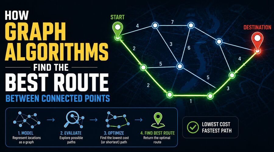

Finding the best route between two connected points is one of the most common problems in computer science. Whether a navigation app is choosing the fastest road to a destination, a delivery company is planning efficient routes, a computer network is directing data packets, or a game character is moving through a virtual world, the underlying problem can often be represented using a graph. 🔗
A graph is a mathematical structure made of vertices, also called nodes, and edges, which represent the connections between them. Once a real-world system is converted into a graph, specialized algorithms can analyze the network and determine the most efficient path from one node to another.
These methods are known as graph algorithms, and several of them are specifically designed to solve shortest-path and route-finding problems.
🔗 What Is a Graph?
In graph theory, a graph consists of two main components:
- Vertices or nodes represent individual points.
- Edges represent connections between those points.
Imagine a road map. Each city can be represented as a node, while each road connecting two cities becomes an edge.
For example:
City A → City B → City C
If there is also a direct road from City A to City C, the graph contains another edge between those two nodes.
Graphs can represent far more than roads. They can model:
- 🌐 Internet networks
- 🏙️ City transportation systems
- ✈️ Airline routes
- 🚆 Railway networks
- 👥 Social networks
- 🎮 Game maps
- 🧬 Biological networks
- 📦 Logistics systems
Once these systems are represented as graphs, algorithms can search them systematically.
⚖️ Weighted and Unweighted Graphs
Not all routes are equally desirable.
A road between two cities may be 20 kilometers long while another is 80 kilometers long. One network connection may take 10 milliseconds while another takes 100 milliseconds.
To represent these differences, graph edges can have weights.
A weight is a numerical value associated with an edge.
For a road network, the weight could represent:
- Distance
- Travel time
- Fuel consumption
- Toll cost
- Traffic congestion
For computer networks, a weight could represent:
- Latency
- Bandwidth cost
- Network congestion
- Transmission reliability
A graph containing these values is called a weighted graph.
In an unweighted graph, every connection is treated equally.
This distinction determines which routing algorithm is most appropriate.
🧭 What Does “Best Route” Actually Mean?
The best route is not always simply the physically shortest route.
Different applications may define “best” differently.
A navigation application might search for the route with the lowest travel time rather than the lowest distance.
A logistics system might prioritize fuel efficiency.
A computer network might try to minimize communication delay.
An emergency vehicle routing system could prioritize roads with the lowest expected congestion.
Mathematically, the problem usually becomes:
Find the path between a starting node and destination node whose total cost is as small as possible.
The total cost is calculated by adding the weights of the edges along the route.
For example, suppose there are two possible paths:
Route 1: A → B → D
Cost: 4 + 3 = 7
Route 2: A → C → D
Cost: 2 + 9 = 11
If the objective is to minimize cost, Route 1 is better.
Graph algorithms perform this comparison automatically, even when a network contains millions of nodes and connections.
🔍 Breadth-First Search for Simple Routes
One of the simplest graph-search algorithms is Breadth-First Search, commonly called BFS.
BFS is especially useful for finding the shortest path in an unweighted graph.
The algorithm begins at the starting node and explores all neighboring nodes first.
It then explores the neighbors of those nodes, continuing outward level by level.
Imagine dropping a stone into water. 🌊
Ripples spread outward evenly from the point where the stone lands.
Breadth-First Search behaves similarly. It expands through the graph one layer at a time.
If every edge has equal cost, the first time BFS reaches the destination, it has found the route containing the fewest edges.
BFS is useful for problems such as:
- Finding the minimum number of connections between users in a social network
- Solving simple maze problems
- Finding minimum steps in certain games
- Exploring communication networks
However, BFS is not suitable when edges have different costs.
For weighted graphs, more advanced algorithms are required.
🚦 Dijkstra’s Algorithm
One of the most famous shortest-path algorithms is Dijkstra’s algorithm.
It was developed by computer scientist Edsger W. Dijkstra and is widely used for finding shortest paths in graphs where edge weights are nonnegative.
The basic idea is straightforward.
The algorithm begins at the starting node and assigns it a distance of zero.
Every other node initially receives an infinite distance because no route to those nodes has yet been discovered.
The algorithm then repeatedly selects the unvisited node with the smallest known distance.
From that node, it examines neighboring nodes and checks whether traveling through the current node provides a cheaper route.
This process is called relaxation.
🔄 How Edge Relaxation Works
Suppose the algorithm knows that reaching Node B from Node A costs 5.
There is an edge from B to C with a cost of 3.
The algorithm therefore calculates:
5 + 3 = 8
If the previously known cost of reaching C was 12, the algorithm updates it to 8.
In other words, it has discovered a better route.
This comparison continues until the shortest paths have been determined.
A simplified network might look like this:
A → B = 4
A → C = 10
B → C = 3
At first, the direct route from A to C appears to cost 10.
But Dijkstra’s algorithm discovers that:
A → B → C = 4 + 3 = 7
Therefore, the indirect route is actually better.
This ability to repeatedly improve route estimates makes Dijkstra’s algorithm extremely powerful.
📊 Priority Queues Make Dijkstra Faster
Efficient implementations of Dijkstra’s algorithm usually use a data structure called a priority queue.
The priority queue keeps track of which node currently has the smallest known distance.
Instead of repeatedly searching every node, the algorithm can quickly select the most promising node to process next.
A common implementation uses a binary heap.
For many graph representations, Dijkstra’s algorithm can run approximately in:
O((V + E) log V)
where:
- V is the number of vertices
- E is the number of edges
This efficiency makes it practical for many large routing systems.
⭐ A* Search: Using Knowledge About the Destination
Dijkstra’s algorithm searches outward based entirely on known path costs.
But what if the algorithm also has information about where the destination is located?
That is where the A* algorithm, pronounced “A-star,” becomes useful.
A* combines two values:
f(n) = g(n) + h(n)
where:
- g(n) is the actual cost from the starting node to the current node
- h(n) is an estimated cost from the current node to the destination
- f(n) is the estimated total route cost
The estimated component, h(n), is called a heuristic.
For geographic navigation, the heuristic might be the straight-line distance from the current location to the destination.
This allows A* to focus its search toward promising areas instead of exploring equally in every direction. 🎯
🗺️ Why A* Is Popular in Maps and Games
Imagine searching for a path across a large city.
Dijkstra’s algorithm may examine roads extending in many directions from the starting point.
A* can use the destination’s approximate position to prioritize roads leading toward it.
This often reduces the number of nodes that need to be examined.
A* is therefore widely used in:
- 🎮 Video game pathfinding
- 🤖 Robot navigation
- 🗺️ Geographic routing systems
- 🧩 Puzzle solving
- 🚚 Logistics planning
The quality of the heuristic plays an important role.
If the heuristic never overestimates the true remaining cost, A* can still guarantee an optimal route under appropriate conditions.
➖ What About Negative Edge Weights?
Dijkstra’s algorithm assumes that edge weights are nonnegative.
But some graphs contain negative values.
For example, a financial model might represent profit as a negative cost.
In such cases, Dijkstra’s algorithm may produce incorrect results.
A different algorithm called the Bellman-Ford algorithm can handle graphs containing negative edge weights.
Bellman-Ford repeatedly relaxes every edge in the graph.
It is generally slower than Dijkstra’s algorithm, but it has an important advantage: it can detect negative-weight cycles.
A negative-weight cycle is a loop whose total cost is negative.
If such a cycle exists and can be repeatedly traveled, there may be no meaningful shortest path because the total cost can continue decreasing indefinitely.
🌍 Finding Routes Between Many Points
Sometimes a system needs more than a single route between two nodes.
It may need shortest-path information between every pair of nodes.
One algorithm designed for this problem is the Floyd-Warshall algorithm.
Instead of searching from one starting point, Floyd-Warshall systematically compares possible intermediate nodes.
Its time complexity is approximately:
O(V³)
That makes it expensive for extremely large graphs, but it can be useful when the graph is relatively small and shortest paths between many node pairs are required.
🚗 How Navigation Systems Represent Roads
Real navigation systems are far more complex than simple textbook graphs.
A road intersection may become a node, while road segments become edges.
Each edge can contain detailed information such as:
- Road distance
- Typical travel time
- Current traffic speed
- Speed limits
- Road restrictions
- Toll information
- Turn restrictions
- Vehicle access rules
- Road closures
The route-finding algorithm then assigns costs based on these factors.
For example, a highway route may be longer in distance but faster in travel time.
If the user selects “fastest route,” the system may choose the highway.
If the user selects “avoid tolls,” toll roads can be given a very high cost or excluded entirely.
This demonstrates an important idea: graph algorithms optimize whatever cost function they are given.
🚦 Dynamic Routing and Traffic
Real roads constantly change.
Traffic accidents, construction, weather, and rush-hour congestion can alter travel times.
Modern navigation systems therefore use dynamic edge weights.
If a road normally takes 10 minutes but current traffic increases that estimate to 25 minutes, its edge weight can be updated.
The routing system can then calculate a new path.
This is why navigation apps may suddenly recommend leaving a highway and taking another route.
The underlying graph may be the same, but its edge weights have changed.
🌐 Routing on the Internet
Graph algorithms are also fundamental to computer networking.
Routers can be represented as nodes, while communication links become edges.
Routing protocols analyze these networks to determine how information should travel.
A path might be selected based on:
- Network delay
- Link cost
- Number of hops
- Reliability
- Available bandwidth
For example, link-state routing protocols use ideas closely related to shortest-path algorithms.
Routers construct a representation of network topology and calculate efficient paths through it.
Every time you access a website, send a message, or stream a video, routing decisions help move data through interconnected networks. 🌐📡
🤖 Graph Algorithms in Robotics
Autonomous robots also need efficient pathfinding.
A robot operating inside a warehouse might represent intersections and movement corridors as a graph.
The robot could then use A*, Dijkstra’s algorithm, or related techniques to determine a safe route toward a storage location.
However, robotic navigation adds extra challenges.
The system may need to consider:
- Obstacles
- Turning radius
- Battery consumption
- Collision risks
- Moving objects
- Restricted zones
The “shortest” route may therefore not necessarily be the best route.
A slightly longer path might consume less energy or provide greater safety.
🎮 Graph Algorithms in Video Games
Video games often rely heavily on pathfinding.
Non-player characters must navigate around walls, buildings, terrain, and other obstacles.
A game environment can be transformed into a graph using grid cells, navigation meshes, or predefined waypoints.
The pathfinding algorithm then calculates how a character should move.
A* is especially popular because its heuristic helps concentrate the search toward the target.
Without efficient graph algorithms, characters might take unnecessarily long routes, become stuck, or consume too much computing power while searching.
📦 Delivery and Logistics Optimization
Package delivery provides another major application.
A delivery vehicle may need to visit dozens or hundreds of destinations.
Finding the shortest route between two locations is relatively straightforward compared with determining the best route through many destinations.
This leads to more complicated optimization problems such as the Traveling Salesperson Problem and Vehicle Routing Problem.
For large systems, finding the mathematically perfect solution can be computationally expensive.
Companies therefore combine graph algorithms with optimization methods and heuristics to create highly efficient practical routes.
These systems may consider:
- Delivery deadlines
- Vehicle capacity
- Driver schedules
- Traffic conditions
- Fuel or electricity consumption
- Depot locations
Graph theory provides the fundamental structure on which these larger optimization systems are built.
🧠 Why Choosing the Right Algorithm Matters
Different graph algorithms are suited to different situations.
Breadth-First Search works well when every connection has equal cost.
Dijkstra’s algorithm works well when edges have nonnegative weights.
A* is useful when a good estimate of the remaining distance is available.
Bellman-Ford can handle negative edge weights.
Floyd-Warshall can calculate shortest paths between all pairs of nodes.
There is therefore no single graph algorithm that is automatically best for every routing problem.
Engineers must consider graph size, edge properties, memory limitations, update frequency, and the type of answer required.
⚡ Scaling to Massive Networks
Real-world graphs can contain millions or even billions of nodes and edges.
Running a basic shortest-path algorithm across the entire network for every request may be inefficient.
Large navigation systems therefore use advanced optimization techniques.
These can include:
- Bidirectional search
- Graph partitioning
- Hierarchical routing
- Precomputed distances
- Landmark-based heuristics
- Route caching
Bidirectional search, for example, can search outward from both the starting point and destination until the two searches meet.
Hierarchical routing can treat major highways differently from smaller local streets, reducing the number of roads that need to be considered during long-distance journeys.
These techniques help modern systems answer routing queries extremely quickly.
🔬 Graph Algorithms and Artificial Intelligence
Graph algorithms also intersect with artificial intelligence.
Machine learning may predict future traffic conditions, while graph algorithms use those predictions to calculate routes.
AI systems can estimate:
- Future travel times
- Congestion patterns
- Accident risks
- Delivery demand
- Energy consumption
These predicted values can then become edge weights in a routing graph.
The graph algorithm still performs the path calculation, while machine learning improves the information used to make that decision.
This combination is becoming increasingly important in autonomous transportation, smart cities, and logistics. 🤖🌆
✨ Conclusion
Graph algorithms find the best route between connected points by representing a system as nodes and edges and then systematically comparing possible paths.
The meaning of “best” depends on the application. It might refer to the shortest distance, fastest travel time, lowest fuel consumption, minimum network delay, or another measurable cost.
Algorithms such as Breadth-First Search, Dijkstra’s algorithm, A*, Bellman-Ford, and Floyd-Warshall solve different versions of this routing problem.
Dijkstra’s algorithm gradually expands from the starting point while keeping track of the lowest known costs. A* improves the process by using a heuristic to guide the search toward the destination. Other algorithms handle unusual conditions such as negative edge weights or the need to calculate routes between many points.
These concepts may appear mathematical, but they have enormous practical importance. Every time a navigation app chooses a road, a game character moves toward a target, a robot travels through a warehouse, or a network directs information across the internet, graph algorithms may be working behind the scenes. 🗺️💻
By turning complicated networks into structured mathematical graphs, computers can compare thousands or millions of possible connections and find efficient routes remarkably quickly. That makes graph algorithms one of the most powerful foundations of modern navigation, networking, logistics, robotics, and computer science.