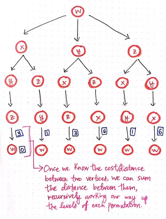
In order to determine which of these six possible paths is the shortest one — and thus the ideal choice for our salesman — we need to build up the cost of every single one of these paths.
Calculating recursive costs using recursion for TSP, part 1.
Since we’ve used recursion to expand these paths until we hit our base case of “no more nodes left to visit”, we can start to close up these recursive calls, and calculate the cost of each path along the way.
Once we know the cost between two vertices, we can sum the distance between them, and the remove the node from the tree. This will make more sense with an example, so let’s work our way from the lowest-level of this tree until we have found a solution for the shortest path.
We know that every single one of these branches — each of which represents a permutation of this particularly problem — ends with the node that we started on: node w. We’ll start with node w, and calculate the cost for our salesman to travel there.
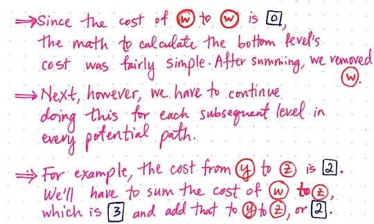
Well, since our salesman starts at node w, the cost of traveling to node w is actually just 0. This makes sense if we think about it, because our salesman is already at that vertex, so it isn’t going to “cost” him anything to travel there! So, the math for the bottom level is pretty easy — the cost to get from w to w is 0. Next, we’ll apply the same technique again, but this time, we’ll move one level up.
Understanding the logic behind recursive addition for TSP.
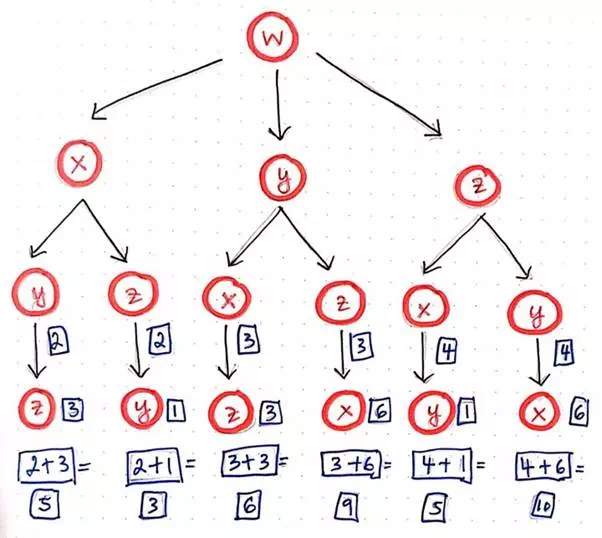
For example, if we refer to our adjacency matrix from the previous section, we’ll see that the cost of traveling from w to z is 3. Since we’re traveling from w —> w —> z, we can sum the distances between each of these vertices as we go. Traveling from w —> w is 0, and traveling from w —> z is 3, so we are essentially calculating 0 + 3. In a similar vein, the cost from z to y is 2. So, we will need to calculate w —> w —> z -> y, which is 0 + 3 + 2.
The drawing below illlustrates how this addition slowly works its way up the tree, condensing the recursive calls that built it up in the first place.
Calculating recursive costs using recursion for TSP, part 2.
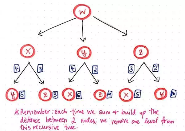
Through this process, we’re effectively building up the cost or distance of each path, one level at a time, using our tree structure. Each time that we sum the distance between two nodes, we can remove the bottom node (the deeper of the two nodes being added together) from the tree, since we don’t need to use it anymore.
Calculating recursive costs using recursion for TSP, part 3.
It is worth mentioning that we need to keep track of each of these paths, even after we finish doing the work of adding up their costs. For the sake of brevity, the paths themselves are not included in the illustrations shown here. However, it is crucial to keep track of which nodes were at the bottom of the tree — otherwise, we’d lose the entire path itself!
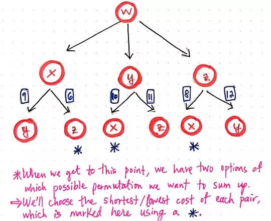
We will continue this process, but at some point, an odd thing is going to happen. In the next iteration of this recursive addition, we’ll notice that we come to an interesting fork in the road — literally! When we reach the third level and have condensed the bottom part of the tree, we have two possible options of how we can proceed with our additon.
Calculating recursive costs using recursion for TSP, part 4.
For example, looking at the child paths/branches from node x, we could either sum the distance from x to y, or we could sum the distance from x to z. So, how do we decide which one to choose?
Calculating recursive costs using recursion for TSP, part 5.
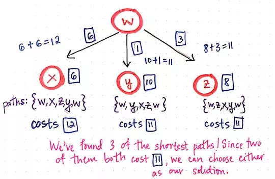
Our gut instinct would tell us that we’re looking for the shortest path, which probably means that we’ll want to choose the smaller of the two values. And that’s exactly what we’ll do! We’ll choose the path from z leading back to x, since the cost of that path is 6, which is definitely smaller than the path from y leading back to x, which is 9.
Once we’ve chosen the smallest of the two paths in our “fork in the road”, we are left with just three paths. All that’s left to do is to figure out the total cost of from x to w, y to w, and z to w. Referring to our adjacency matrix, we’ll see that these distances are 6, 1, and 3, respectively.
We can add these to the total costs of the paths that we’ve been recursively summing this whole time. In the illustration above, we’ll see that the three shortest paths that we’ve determined are actually noted down for convenience. As it turns out, there is one path that costs 12, and two paths that both cost 11. One of those travels from w to y, and takes the route of w -> y -> x -> z -> w, while the other travels from w to z, and takes the route of w -> z-> x -> u -> w.
Since two of our three paths are equivalently small in size, it doesn’t really matter which one we choose; both of them are the “shortest path” in solving the traveling salesman problem.
And there we have it! We’ve solved for a Hamiltonian circuit by finding the shortest path, with a distance/cost of 11, that starts and ends at node w.
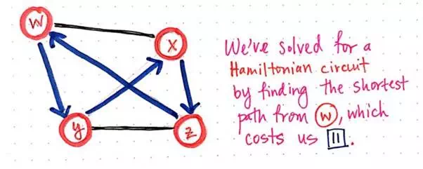
We’ve solved for a Hamiltonian circuit!
Solving that was pretty awesome, right? It seemed super daunting at first, but as we worked through it, it got easier with each step. But here’s the thing: we had to take a lot of steps to do this. We knew from the beginning that we weren’t going to have the most elegant solution to this problem — we were just trying to get something working. But just how painful is the brute-force method, exactly?
Well, what if instead of a salesman who has to travel to four cities, we were trying to help out a salesman who had to travel to a whole lot more cities? What if the number of cities that they had to visit was n? How bad would our brute-force technique be?
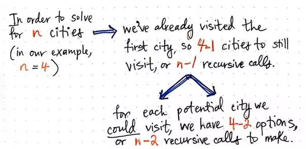
Well, in our first example, n = 4. We’ll recall that, since we had already visited our first city (node w), we only had to make three recursive calls. In other words, we had to make 4 — 1, or n — 1 recursive calls.
Solving for n cities in the TSP.
But, for each of those recursive calls, we had to spawn off two more recursive calls! That is to say, for each potential city that we could visit from the three nodes x, y, and z, we had 4 — 2 = 2 options of paths to take. In abstract terms, we’d effectively have n — 2 recursive calls at the next level of our tree.
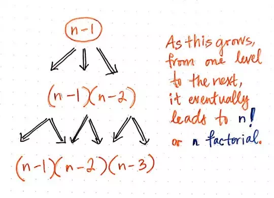
Building up an unscalable “n factorial” problem.
If we continue figuring out this math, we’ll see that, at each level of the tree, we are basically on the path to finding a number that is going to be a factorial. To be more specific, we’re going to end up with n!, or n factorial.
Now, when we were dealing with a salesman who needed to visit just four cities, this really wasn’t too terrible of scenario to deal with. But, what happens when nis something much, much larger than 4? Most salesmen and women aren’t going to be traveling just to four cities; in almost every realistic case, n is going to be a much larger number!
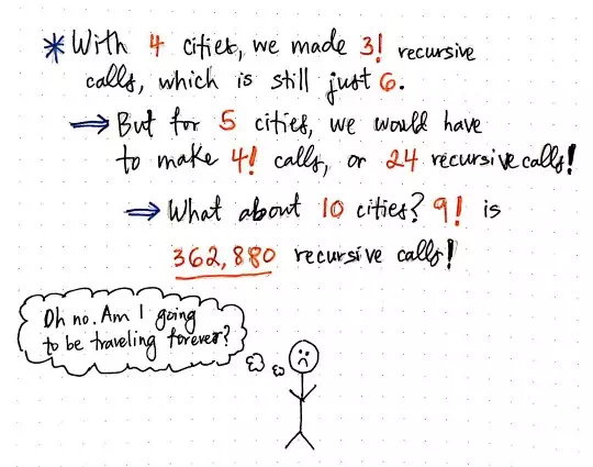
The traveling salesman is not a fan of factorial algorithms!
Well, to get a sense of how unscalable a factorial algorithm is, we needn’t increase the value of n by all that much. For example, when n = 4, we made 3! or 6recursive calls. But if we had increased this only slightly so that n = 5, we would make 4! or 24 recursive calls, which would lead to a much, much larger tree. And what about when n = 10? That would result in 9! recursive calls, which is a really huge number: 362,880 to be exact. We probably can’t even imagine what would happen if our salesman had to travel to every city in the country, or even just 10 cities for that matter!
Surely, there must be a better way of helping our traveling salesman out so that he’s not traveling forever? Well, there certainly is. But more on that next week. In the meantime, someone should really tell this salesman about eBay — it would probably save him a whole lot of heartache!


