Interactions within a Distributed System between 2 processes, P1 and P2.
Distributed systems offer us the ability to solve problems we couldn’t possibly solve with a single machine. However, I have recently become painfully aware that every solution to a problem brings with it a series of new problems and considerations to be made.
Within the realm of distributed systems, one of the largest problems we gain over a single machine system is attempting to keep a correct timeline of events. This is needed for a variety of reasons — one of the most crucial is understanding the ordering and causality of events within your system. This is what allows analysis to be performed when evaluating why your system executed a specific action.
For instance, if you want to know why a particular value was written to your database, you may search for the series of events leading up to the point of the INSERT request being created. You can then place these events in chronological order using their timestamp, traversing from latest → oldest in order to understand the causality of actions leading up to the final value being written [Figure 1].
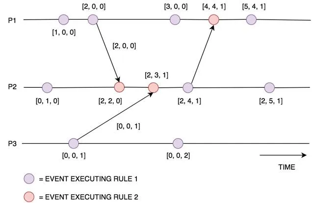
Figure 1 : this shows a series of events by a single process [P1], leading up to a database INSERT request being made. You can see that using timestamps allow the events to be placed in chronological order, showing how the variable V ended up assuming the value 6 when sent to the database.
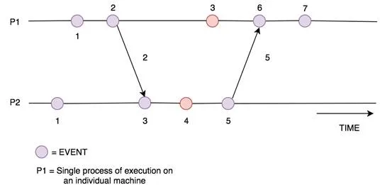
When we have a single machine, a timeline of events is relatively easy to create, even if we have multiple processes (threads) creating events. This is due to all the events, across processes, sharing the same Physical Clock. When each one of those events logs the time in which it executed, we can guarantee when constructing a timeline that all events will be placed in the correct order with respect to each other. This is due to the same Physical Clock being used for all timestamps, providing a single global view of time [Figure 2].
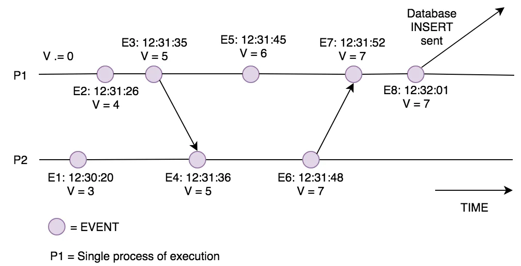
Figure 2: this shows 2 processes sending messages between each other affecting the variable V. You can see that the timestamps still work as they are both on the same machine with the same single view of time. Thus, we can order the events and determine what caused V to be equal to 7 when it was sent to the database.
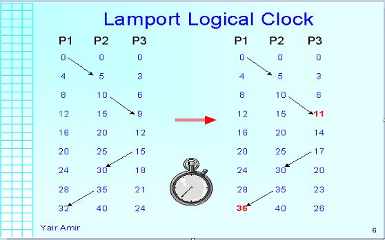
However, when we move to a distributed system we cannot rely on this property anymore. Let’s take our previous example to prove this. If we have events leading up to an INSERT now happening across multiple machines, each with their own local clock, and we use timestamps to place events in chronological order, we now have to guarantee that every machines clock has the exact same time. This is known as having a Global Clock, and is not easily achieved in a distributed system [Figure 3].
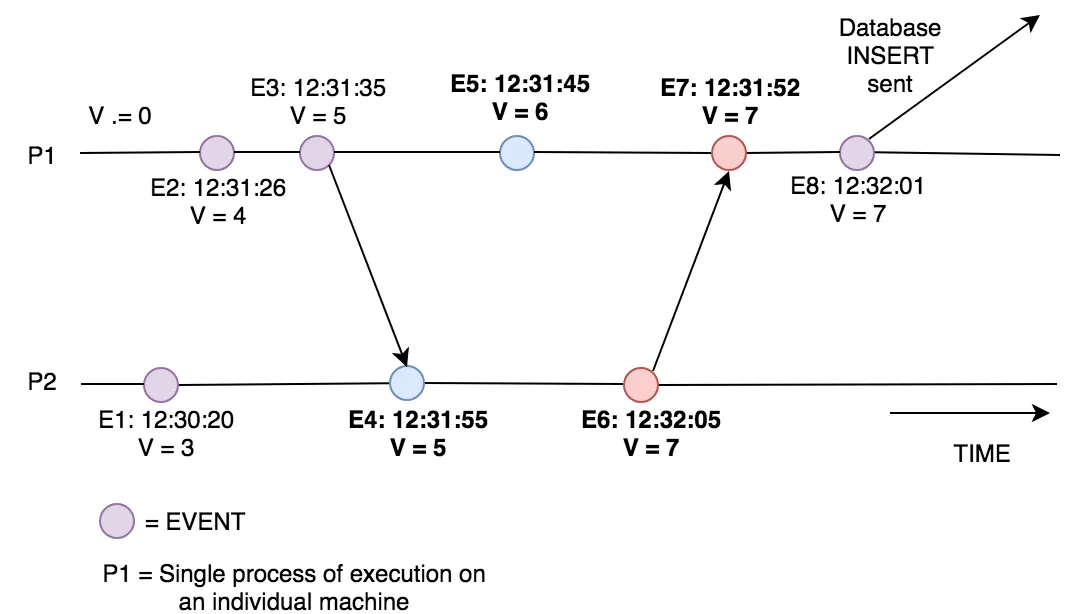
Figure 3: the above diagram shows the inconsistent states we can get into if there is no global clock. You can see the clocks within P1 and P2 differ enough for us to get incorrect ordering of events. We think E4 happens after E5 (blue) based on the timestamps only. We also see that E6 was sent after it arrives in P1 at E7 (red). This makes the system impossible to draw causality from when investigating the database INSERT event.
Instead, a distributed system really has an approximation of the Physical Time across all its machines. An approximation may be good enough if events happen infrequently, as you will always be able to place events into the correct chronological order as long as the clocks of every machine stay synchronized within some acceptable threshold. Though, in most distributed systems this is not a good enough guarantee. Therefore, we have to look to a virtual way of expressing time between machines, so we can keep the ability to place events into an accurate timeline. This is the notion of Logical Clocks.
Logical Clocks refer to implementing a protocol on all machines within your distributed system, so that the machines are able to maintain consistent ordering of events within some virtual timespan. This is more formally specified as a way of placing events in some timespan so the following property will always be true:
Given 2 events (e1, e2) where one is caused by the other (e1 contributes to e2 occurring). Then the timestamp of the ‘caused by’ event (e1) is less than the other event (e2).
To provide this functionality any Logical Clock must provide 2 rules:
Rule 1: this determines how a local process updates its own clock when an event occurs.
Rule 2: determines how a local process updates its own clock when it receives a message from another process. This can be described as how the process brings its local clock inline with information about the global time.
The simplest implementation of this is Scalar Time. In this representation each process keeps a local clock which is initially set to 0. It then provides the following implementation of the 2 rules:
Rule 1: before executing an event (excluding the event of receiving a message) increment the local clock by 1.
local_clock = local_clock + 1
Rule 2: when receiving a message (the message must include the senders local clock value) set your local clock to the maximum of the received clock value and the local clock value. After this, increment your local clock by 1 [Figure 4].
1. local_clock = max(local_clock, received_clock)
2. local_clock = local_clock + 1
3. message becomes available.
Figure 4: the above diagram shows how using Scalar Time, the 2 processes (P1 and P2) update their local clocks based on the messages they receive.
We can see that Scalar Time provides an eventually consistent state of time. This means there may be places where the recorded time differs between processes but, given a finite amount of time, the processes will converge on a single view of the correct time. Causing this is the fact that internal events in a process (that apply Rule 1) loose consistency with regards to concurrent events on another process (red events in Figure 4). This is due to the use of a single number for both our global and local clocks across processes. In order to become causally consistent we need a way of representing local time and global time separately. This is where Vector Clocks come in.
Vector Clocks expand upon Scalar Time to provide a causally consistent view of the world. This means, by looking at the clock, we can see if one event contributed (caused) another event. With this approach, each process keeps a vector (a list of integers) with an integer for each local clock of every process within the system. If there are N processes, there will be a vector of N size maintained by each process. Given a process (Pi) with a vector (v), Vector Clocks implement the Logical Clock rules as follows:
Rule 1: before executing an event (excluding the event of receiving a message) process Pi increments the value v[i] within its local vector by 1. This is the element in the vector that refers to Processor(i)’s local clock.
local_vector[i] = local_vector[i] + 1
Rule 2: when receiving a message (the message must include the senders vector) loop through each element in the vector sent and compare it to the local vector, updating the local vector to be the maximum of each element. Then increment your local clock within the vector by 1 [Figure 5].
1. for k = 1 to N: local_vector[k] = max(local_vector[k], sent_vector[k])
2. local_vector[i] = local_vector[i] + 1
3. message becomes available.
Figure 5: the above diagram shows how the vector clocks are updated when executing internal events, sending events and receiving events. It also shows the values of the vectors sent between processes.
Vector Clocks provide a causally consistent ordering of events, however this does come at a price. You can see that we need to send the entire Vector to each process for every message sent, in order to keep the vector clocks in sync. When there are a large number of processes this technique can become extremely expensive, as the vector sent is extremely large. There have been many improvements over the initial Vector Clock implementation mentioned, most notably:
· Singhal–Kshemkalyani’s differential technique [1]: This approach improves the message passing mechanism by only sending updates to the vector clock that have occurred since the last message sent from Process(i) → Process(j). This drastically reduces the message size being sent, but does require O(n²) storage. This is due to each node now needing to remember, for each other process, the state of the vector at the last message sent. This also requires FIFO message passing between processes, as it relies upon the guarantee of knowing what the last message sent is, and if messages arrive out of order this would not be possible.
· Fowler-Zwaenepoel direct-dependency technique [2]: This technique further reduces the message size by only sending the single clock value of the sending process with a message. However, this means processes cannot know their transitive dependencies when looking at the causality of events. In order to gain a full view of all dependencies that lead to a specific event, an offline search must be made across processes.