The traveling salesman in our example problem has it pretty lucky — he only has to travel between four cities. For simplicity’s sake, we’ll call these four cities w, x, y, and z. Because we know that TSP is a graph problem, we can visualize our salesman’s possible routes in the form of a weighted, undirected graph. We’ll recall that a weighted graph is one whose edges have a cost or distance associated with them, and an undirected graph is one whose edges have a bidirectional flow.

Looking at an illustrated example of our salesman’s graph, we’ll see that some routes have a greater distance or cost than others. We’ll also notice that our salesman can travel between any two vertices easily.

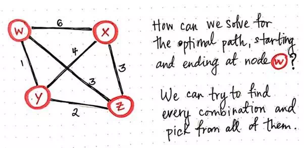
How can we solve for the optimal path starting and ending at node w?

Let’s say that our salesman lives in city w, so that’s where he’ll start his journey from. Since we’re looking for a Hamiltonian cycle/circuit, we know that this is also where he will need to end up at the end of his adventures. So, how can we solve for the optimal path so that our salesman starts and ends at city (node) w, but also visits every single city (x, y, and z) in the process?

Remember, we’re not going to think about the most efficient strategy — just one that works. Since we’re going to use the brute-force approach, let’s think about what we’re really trying to solve for here. The brute-force approach effectively means that we’ll solve our problem by figuring out every single possiblity and then picking the best one from the lot. In other words, we want to find every single permutation or possible path that our salesman could take. Every single of one of these potential routes is basically a directed graph in its own right; we know that we’ll start at the node w and end at w, but we just don’t know quite yet which order the nodes x, y, and z will appear in between.

Every permutation is, on its own, a directed graph.

So, we need to solve every single possible combination to determine the different ways that we could arrange x, y, and z to replace the nodes that are currently filled with ?’s. That doesn’t seem too terrible.

But how do we actually solve for these ? nodes, exactly? Well, even though we’re using a less-than-ideal brute-force approach, we can lean on recursion to make our strategy a little more elegant.

The basic idea in the recursive TSP approach is that, for every single node that we visit, we keep track of the nodes that we can navigate to next, and then recursively visit them.

Eventually, we’ll end up with no more nodes to check, which will be our recursive base case, effectively ending our recursive calls to visit nodes. Don’t worry if this seem complicated and a little confusing at the moment; it will become a lot clearer with an example. So, let’s recursively brute-force our way through these cities and help our salesman get home safe and sound!

We already know that our salesman is going to start at node w. Thus, this is the node we’ll start with and visit first. There are two things we will need to do for every single node that we visit — we’ll need to remember the fact that we’ve visited it, and we’ll need to keep track of the nodes that we can potentially visit next.

Generating recursive calls for TSP, part 1.

Here, we’re using a list notation to keep track of the nodes that we can navigate to from node w. At first, we can navigate to three different places: {x, y, z}.

Recall that recursion is basically the idea that a “function calls itself from within itself”. In other words, as part of solving this problem, we’re going to have to apply the same process and technique to every single node, again and again. So that’s exactly what we’ll do next! For every single node that we can potentially navigate to, we will recursively visit it.

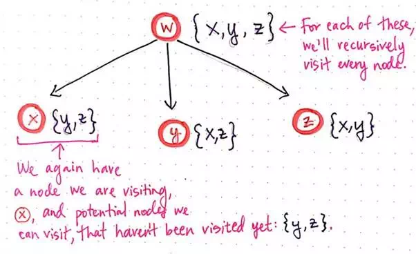
Generating recursive calls for TSP, part 2.

Notice that we’re starting to create a tree-like structure. For each of the potential nodes to visit from the starting node w, we now have three potential child “paths” that we could take. Again, for each of these three vertices, we’re keeping track of the node itself that we’re visiting as well as any potential nodes that we can visit next, which haven’t already been visited in that path.

Recursion is about repetition, so we’re going to do the same thing once again! The next step of recursion expands our tree once again.

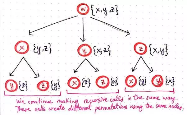
Generating recursive calls for TSP, part 3.

We’ll notice that, since each of the three nodes x, y, and z had two nodes that we could potentially visit next, each of them have spawned of two of their own recursive calls. We’ll continue to make recursive calls in the same way and, in the process, we’ll start to see that we’re creating different permutations using the same nodes.

We’ll notice that we’re now at the third level of recursive calls, and each node has only one possible place to visit next. We can probably guess what happens next — our tree is going to grow again, and each of the bottom-level nodes is going to spawn a single recursive call of its own, since each node has only one unvisited vertex that it can potentially check.

The image shown below illustrates the next two levels of recursive calls.

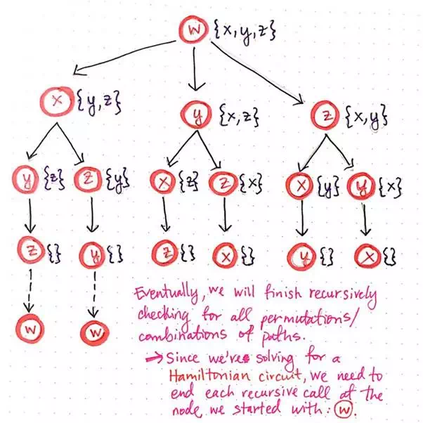
Generating recursive calls for TSP, part 4.

Notice that, when we get to the fourth level of child nodes, there is nowhere left to visit; every node has an empty list ({} ) of nodes that it can visit. This means that we’ve finished recursively checking for all permutations of paths.

However, since we’re solving for a Hamiltonian cycle, we aren’t exactly done with each of these paths just yet. We know we want to end back where we started at node w, so in reality, each of these last recurisvely-determined nodes needs to link back to vertex w.

Once we add node w to the end of each of the possible paths, we’re done expanding all of our permutations! Hooray! Remember how we determined earlier that every single of one of these potential routes is just a directed graph? All of those directed graphs have now revealed themselves. If we start from the root node, w, and work down each possible branch of this “tree”, we’ll see that there are six distinct paths, which are really just six directed graphs! Pretty cool, right?

So, what comes next? We’ve expanded all of these paths…but how do we know which one is the shorted one of them all?

We haven’t really been considering the cost or distance of this weighted graph so far, but that’s all about to change. Now that we’ve expanded this problem and found all of its possible permutations, we need to consider the total cost of each of these paths in order to find the shortest one. This is when an adjacency matrix representation of our original graph will come in handy. Recall that an adjacency matrix is a matrix representation of exactly which nodes in a graph contain edges between them. We can tweak our typical adjacency matrix so that, instead of just 1’s and 0’s, we can actually store the weight of each edge.

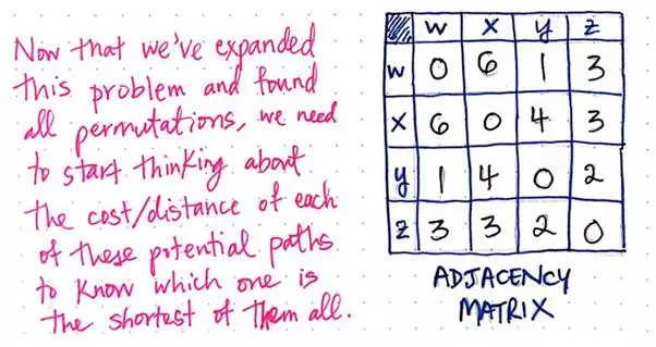
We can use an adjacency matrix to help us keep track of edge costs/distances.

Now that we have an adjacency matrix to help us, let’s use it to do some math — some recursive math, that is!