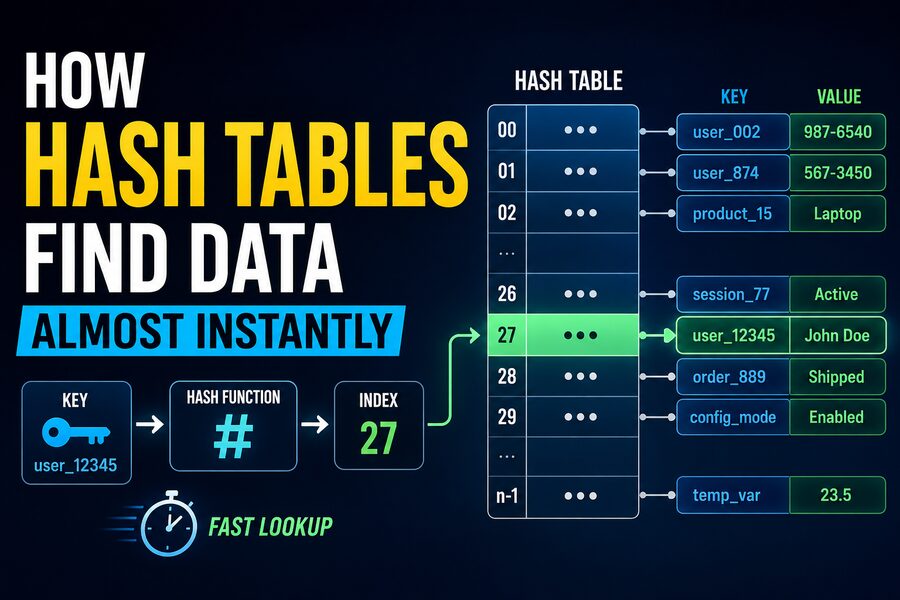

When you search for a username in an app, look up a product by ID, check whether a word exists in a dictionary, or retrieve information from a database, the result often appears almost instantly. Behind many of these fast lookups is a remarkably efficient computer science structure called a hash table. 💻
Hash tables are designed to store and retrieve data quickly by transforming a key—such as a name, number, or identifier—into a location where the corresponding value can be found.
Instead of checking every stored item one by one, a hash table tries to jump directly to the correct location.
That is why hash tables can often find information in approximately constant time, written in computer science as O(1) average-case lookup time.
The secret lies in a mathematical tool called a hash function. 🔢
🗂️ Why Searching Normally Can Be Slow
Imagine you have a list containing one million customer records.
Each record includes a customer ID and account information.
If the records are stored in an ordinary unsorted list and you need to find customer ID 583291, the computer may have to start at the beginning and check each entry:
Is this ID 583291?
No.
What about the next one?
No.
And the next?
This continues until the correct record is found.
In the worst case, the computer could inspect nearly all one million entries.
This type of search has a time complexity of approximately O(n), where n represents the number of stored elements.
As the collection becomes larger, the search generally becomes slower. 🐢
Hash tables use a very different strategy.
🔑 Hash Tables Store Information as Key-Value Pairs
A hash table usually stores information in the form of key-value pairs.
For example:
"alice"→ user account information"SKU-7842"→ product details"France"→"Paris"102938→ customer record
The key is used to locate the information.
The value is the information associated with that key.
This pattern appears throughout computing.
A phone contact list might use a person’s name as the key and their phone number as the value.
A web application might use a session ID as the key and session data as the value.
The challenge is finding the value quickly once the key is known.
That is where hashing begins. ⚙️
🧮 What Is a Hash Function?
A hash function takes a key and converts it into a numerical value called a hash or hash code.
For example, imagine a simplified hash function:
hash("apple") = 42817
The computer can then transform this number into an index in an internal array.
Suppose the hash table contains 100 storage positions.
One simple approach would be:
42817 mod 100 = 17
The value associated with "apple" could therefore be stored at position 17.
Later, when the program needs "apple" again, it performs exactly the same calculation:
"apple" → hash function → 42817 → position 17
Instead of searching through every item, the program jumps directly to position 17. 🎯
This direct mapping is the main reason hash tables are so fast.
📦 Buckets: Where Hash Table Data Lives
Internally, a hash table commonly uses an array divided into storage locations known as buckets or slots.
You can imagine them as numbered containers:
0, 1, 2, 3, 4, 5...
The hash function determines which bucket should hold a particular key.
Suppose we have eight buckets:
0 1 2 3 4 5 6 7
A hash function might send:
"cat"→ bucket 2"dog"→ bucket 6"bird"→ bucket 1"fish"→ bucket 4
If you later ask for "dog", the program hashes "dog" again and immediately checks bucket 6.
There is no need to inspect buckets 0 through 5 first.
This is fundamentally different from sequential searching.
⚡ Why Hash Table Lookup Is Often O(1)
Computer scientists describe hash table operations such as lookup, insertion, and deletion as O(1) on average.
O(1), or constant time, does not literally mean the operation takes exactly the same number of nanoseconds every time.
Instead, it means the amount of work required generally does not grow proportionally with the number of stored items.
Imagine a well-designed hash table containing 100 items.
Finding a key might require calculating its hash and checking one bucket.
Now imagine the table contains 100,000 items.
With good hashing and sufficient capacity, finding a key may still require essentially the same process:
- Compute the key’s hash.
- Determine the bucket.
- Check the bucket.
- Return the value.
That scalability is extremely valuable. 🚀
💥 The Collision Problem
Hash tables have a complication: different keys can sometimes map to the same bucket.
This is called a hash collision.
Suppose the table has 10 buckets.
The hash function produces:
hash("apple") → bucket 3
and:
hash("orange") → bucket 3
Both values cannot simply overwrite one another.
The hash table therefore needs a way to handle collisions.
Collisions are unavoidable because there may be an enormous number of possible keys but only a limited number of buckets.
The goal is not necessarily to eliminate every collision. Instead, a good hash table manages them efficiently. 🛠️
🔗 Collision Handling with Chaining
One common method is called separate chaining.
Instead of allowing each bucket to hold only one item, the bucket can store several entries.
For example:
Bucket 3:
("apple", 25) → ("orange", 41) → ("banana", 72)
When the program looks for "orange", it hashes the key, jumps to bucket 3, and then checks the few entries stored there.
If the hash function distributes keys evenly, each bucket usually contains only a small number of entries.
Lookup therefore remains fast.
Traditionally, chaining has often used linked lists, although implementations may use arrays, trees, or other structures depending on the programming language and design.
➡️ Collision Handling with Open Addressing
Another strategy is known as open addressing.
With open addressing, all entries are stored directly inside the hash table’s array.
If the desired bucket is already occupied, the program searches for another available position according to a predefined rule.
One simple method is linear probing.
Suppose "apple" belongs in bucket 4, but bucket 4 is already occupied.
The program might check:
Bucket 5.
If that is occupied, check bucket 6.
Continue until an available position is found.
Other probing methods include quadratic probing and double hashing.
Each technique attempts to reduce clustering and maintain efficient lookups. 🔍
📊 Why the Load Factor Matters
The performance of a hash table depends heavily on how full it becomes.
A measurement called the load factor describes this relationship.
A simplified formula is:
Load Factor = Number of Stored Entries ÷ Number of Buckets
Suppose a table contains 70 entries and 100 buckets.
Its load factor is:
70 ÷ 100 = 0.70
As a hash table becomes more crowded, collisions become more likely.
More collisions can mean additional work during searches.
To prevent performance from deteriorating, implementations often increase the size of the table when the load factor becomes too high.
📈 What Is Hash Table Resizing?
Imagine a hash table starts with 16 buckets.
As more entries are added, most of those buckets eventually become occupied.
The table may then resize itself to contain perhaps 32 or more buckets.
However, resizing is not simply a matter of adding empty spaces.
Because bucket positions depend on table size, existing keys may need to be placed into new locations.
This process is called rehashing.
Rehashing can temporarily require significant work, but it happens only occasionally.
When the cost is averaged across many insertions, hash table insertion can still achieve approximately O(1) amortized performance.
🎲 What Makes a Good Hash Function?
The quality of the hash function has a major impact on performance.
A good hash function should distribute keys relatively evenly across the available buckets.
Imagine a table with 1,000 buckets.
If nearly every key ends up in bucket 5, the hash table effectively becomes a large list inside one bucket.
Searching could become slow.
A better hash function spreads data across many buckets:
key A → 42
key B → 816
key C → 193
key D → 701
Good distribution reduces collisions and keeps operations efficient.
Hash functions should also be deterministic: the same input must produce the same output whenever the table needs to find that key.
⏱️ Average Case vs. Worst Case
Hash tables are famous for O(1) average lookup, but that does not mean every possible lookup is O(1).
In the worst case, a poorly constructed or heavily collided hash table could degrade toward O(n).
For example, imagine every stored key falls into the same bucket.
Searching that bucket might require checking many entries one by one.
Fortunately, good hash functions, sensible resizing policies, appropriate collision handling, and modern implementation techniques make such extreme behavior uncommon in ordinary use.
This distinction is important:
Average lookup: approximately O(1) ⚡
Worst-case lookup: potentially O(n) 🐢
Some implementations also use additional structures to improve worst-case behavior.
🔐 Hash Tables vs. Cryptographic Hashing
The word “hash” also appears in cybersecurity, but hash tables and cryptographic hashing have different goals.
Hash table hash functions are optimized mainly for:
- Speed
- Deterministic output
- Good distribution
- Efficient indexing
Cryptographic hash functions such as SHA-256 are designed for security-related properties, including making it extremely difficult to reverse or manipulate hashes in useful ways.
A cryptographic hash function is therefore not automatically the best choice for an ordinary hash table.
The concepts are related mathematically, but their engineering objectives differ significantly. 🔒
🆚 Hash Tables vs. Arrays
Arrays are extremely fast when you already know an item’s numerical index.
For example:
array[500]
can directly access position 500.
But what if you want to retrieve information using the key "username_872"?
Arrays do not naturally map arbitrary strings to positions.
A hash table effectively adds that capability by converting arbitrary keys into array-like indexes.
In this sense, hash tables combine the speed of indexed access with the flexibility of meaningful keys.
🌳 Hash Tables vs. Binary Search Trees
Another popular data structure is the balanced binary search tree.
A balanced tree usually provides operations in approximately O(log n) time.
That is slower in theory than a hash table’s average O(1) lookup, although both can be very fast in practice.
Trees have advantages too.
They naturally maintain keys in sorted order.
If you need to ask:
“Give me all values with keys between 100 and 200”
a sorted tree may be very useful.
A normal hash table does not automatically preserve meaningful ordering.
Choosing between them depends on what operations the application needs.
💻 Hash Tables in Programming Languages
Hash tables appear everywhere in modern programming.
Python’s dictionary, or dict, is based on hashing.
Java provides structures such as HashMap.
JavaScript objects have historically provided key-value behavior, while Map offers a dedicated key-value collection.
C++ provides std::unordered_map.
Other programming languages have similar structures known as:
- Dictionaries
- Maps
- Associative arrays
- Hash maps
- Hash sets
Although implementation details differ, the underlying goal is similar: provide extremely fast access to values using keys.
🌐 Where Are Hash Tables Used in Real Life?
Hash tables are useful in an enormous range of software systems.
A web server might use them to manage active user sessions.
A compiler may use a hash table to track variable names.
A game engine might associate entity IDs with objects.
A cache can map requests to previously computed results.
A database system may use hashing internally for certain indexing or query-processing operations.
Operating systems, networking software, browsers, development tools, and cloud platforms all rely heavily on hash-based data structures.
Any time software needs quick “find this exact thing by its key” behavior, a hash table may be a strong candidate. 🌍
🧠 A Simple Real-World Analogy
Imagine a giant hotel with 10,000 numbered mailboxes.
Instead of searching through every mailbox to find a letter for “Alex,” a machine converts the name “Alex” into mailbox number 6,237.
You walk directly to mailbox 6,237 and retrieve the letter.
That is essentially what hashing does.
The name acts as the key.
The conversion rule acts as the hash function.
The mailbox number acts as the bucket index.
And the letter represents the stored value. 📬
If two names happen to map to the same mailbox, the system needs a collision-handling strategy.
Despite that complication, the basic idea remains remarkably efficient.
🚀 Why Hash Tables Feel Almost Instant
The impressive speed of hash tables comes from avoiding unnecessary searching.
Instead of asking:
“Where is this key among millions of possibilities?”
the system asks:
“What location does this key mathematically map to?”
That change turns a potentially long search into a short sequence of operations.
Compute the hash.
Find the bucket.
Check the key.
Return the value.
Modern processors can perform these operations extremely quickly, making hash-based lookup feel instantaneous for many everyday applications.
✅ The Bottom Line
A hash table finds data quickly by using a hash function to convert a key into a storage location.
Instead of scanning every stored item, the computer can jump directly to the bucket where the data is expected to be.
When the hash function distributes keys effectively and the table maintains sufficient capacity, insertion, deletion, and lookup can usually run in approximately O(1) average time.
Collisions are handled through techniques such as chaining or open addressing, while resizing helps prevent the table from becoming overcrowded.
That combination makes hash tables one of the most important data structures in computer science. ⚡💻
Whether you’re logging into an account, loading cached information, looking up a configuration value, or running complex software behind the scenes, there is a good chance a hash table is quietly helping the computer answer the question:
“Where is my data?”
And in many cases, it already knows almost exactly where to look. 🎯