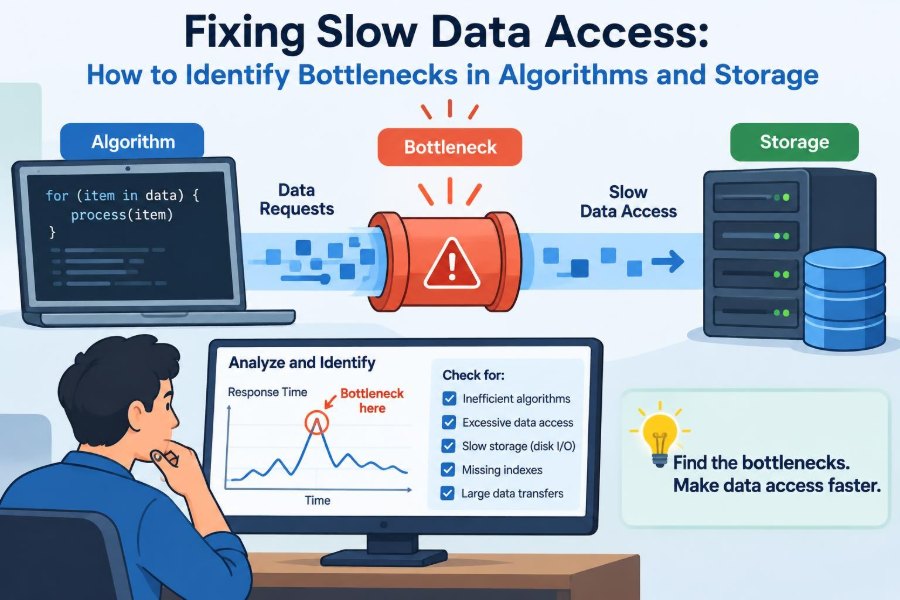

A dashboard that loaded almost instantly last month now takes several seconds. A search box feels sticky. A nightly import runs past the start of the workday. The first instinct is often to blame “the database” or buy faster hardware.
Sometimes storage really is the problem. Just as often, the delay comes from code that asks for too much data, repeats the same lookup thousands of times, sorts a much larger collection than necessary, or waits on a network connection.
Slow data access is frustrating because a single visible delay can be caused by several layers working together: the algorithm, application code, database, cache, file system, network, and physical storage device.
The practical skill is not guessing which layer is at fault. It is learning to measure the path, isolate the slowest part, and make the smallest change that removes the real constraint.
🧭 What “slow data access” actually means
Data access is the work of locating, reading, writing, transferring, and processing information. It can mean finding a record in a database, loading a file, retrieving an object from cloud storage, or reading a value already held in memory.
A request’s latency is the time one operation takes. Throughput is how much work a system completes over time, such as requests per second. A system can have acceptable average latency but poor throughput under load, or high throughput while individual requests still feel slow.
Before changing code, state the symptom precisely: “the report takes 18 seconds,” “p95 search latency rises during imports,” or “writing a batch slows when the table grows.” Precision turns a vague complaint into something testable.
⏱️ Start with a timing boundary
Measure the whole user-visible operation first, then place timers around major stages. For example, time request handling, database execution, result transfer, transformation, rendering, and any external service call.
The goal is a simple timing breakdown, not a mountain of logs. If database execution consumes 80% of the request time, improving HTML rendering will not materially improve the experience. If execution is fast but data transfer is slow, tuning a query plan may miss the real issue.
Use representative inputs. A test with ten records rarely reveals the behavior of a production query over millions of rows or a workload where many users act at once.
🔗 Follow the complete data path
A useful mental model is a pipeline: user action, application logic, connection acquisition, query or file request, storage read, returned bytes, processing, and response. Delay can accumulate at every handoff.
For example, a product page may read an item record quickly, then issue separate queries for inventory, reviews, recommendations, and permissions. Each query may be individually fast, yet the total page remains slow because the waits are sequential.
Tracing tools can attach a timing “span” to each stage of a request. Even without a full tracing platform, structured logs with request IDs and elapsed times can reveal whether slow requests share the same operation.
📏 Distinguish average performance from tail latency
An average hides bad experiences. If nine requests finish quickly and one stalls, the mean may look harmless while one user waits long enough to abandon a task.
Percentiles describe the distribution more clearly. The 95th percentile, often written p95, is a value below which 95% of measured requests completed. Looking at p50, p95, and p99 helps separate ordinary performance from the slow tail.
Tail latency often appears when a cache misses, a disk queue forms, a lock is held, or a shared service becomes busy. Fixing it may require addressing contention rather than merely speeding up normal execution.
🧮 Read algorithmic growth before optimizing details
An algorithm’s time complexity describes how its work tends to grow as input size grows. It does not predict exact seconds, but it explains why code that seems fine in a small test can fail at scale.
Linear work, written O(n), grows roughly with the number of items. Logarithmic work, O(log n), grows slowly as data grows. Quadratic work, O(n²), often comes from comparing every item with many other items and can become expensive surprisingly quickly.
Constants still matter: a linear scan through data already in memory can beat a more complex method for a tiny list. But when data is large or repeatedly accessed, growth rate becomes a decisive design constraint.
🔍 Spot accidental nested scans
A common bottleneck appears when code loops through one collection and searches another collection inside that loop. Suppose an application has orders and customers, then scans the full customer list for each order to find the matching customer.
That pattern can do roughly one lookup per possible order-customer pair. Instead, build a hash map keyed by customer ID once, then retrieve each customer directly while processing orders.
customersById = map customers by customer.id
for each order:
    customer = customersById[order.customerId]
This does not eliminate all cost, but it changes repeated scanning into one preparation pass plus fast lookups. The same principle applies to joining data from files, APIs, and in-memory collections.
🗂️ Choose data structures that match access patterns
A data structure is not just a storage choice; it encodes the operations a program expects to perform. Arrays and lists are useful for ordered traversal. Hash maps are useful for lookup by key. Trees can support ordered searches and range queries.
| Need | Often suitable approach | Trade-off |
|---|---|---|
| Find an item by unique ID | Hash map or database index | Extra memory or write maintenance |
| Read items in order | Sorted structure or ordered index | Inserts may cost more |
| Find values within a range | Tree-based index | Less ideal for arbitrary key lookup |
| Process every item once | Sequential scan | Work grows with collection size |
Do not select a structure solely because it is fast in theory. Consider the data size, read/write ratio, memory limit, ordering needs, and whether the data lives in memory or on disk.
🧾 Understand why database indexes help
A database index is an auxiliary structure that helps locate rows without reading every row in a table. In a rough analogy, it is like an index in a textbook: it helps find a subject without turning every page.
Indexes are most useful for columns used to filter, join, sort, or enforce uniqueness. A query searching for one account by account ID can often avoid a full-table scan when an appropriate index exists.
Indexes are not free. They consume storage, must be updated when indexed data changes, and can make inserts or updates more expensive. An index that does not support a real query pattern may add maintenance without improving useful work.
🧩 Match composite indexes to real queries
Many queries filter on more than one column, such as records for one organization within a date range. A composite index covers multiple columns, but its column order matters.
As a general rule, an index can be most effective when its leading columns align with common equality filters, followed by columns used for ranges or ordering. The exact behavior depends on the database engine and query, so validate with its execution-plan tools.
Creating separate single-column indexes is not always equivalent to creating one useful composite index. The optimizer may combine indexes in some cases, but that can still involve extra work compared with an index shaped for the query.
🧠 Read execution plans instead of guessing
An execution plan is the database’s proposed or actual route for answering a query. It can reveal table scans, index scans, join order, sorting steps, estimated row counts, and operations that spill to temporary storage.
Look for a mismatch between expectation and reality. If a query should return a handful of rows but the plan reads a huge table, investigate missing indexes, broad filters, stale statistics, or a condition that prevents index use.
Plan terminology varies across systems, and a plan is not a verdict by itself. Compare it with measured runtime and rows processed. A full scan can be the right choice for a query that genuinely needs most of a small table.
🧱 Avoid expressions that hide indexed values
A filter may look harmless while making efficient lookup difficult. Applying a function to an indexed column, converting its type, or using a broad wildcard pattern can prevent the database from using the index as intended.
For example, filtering a timestamp by extracting a date may require examining many timestamps. When possible, express the condition as a range: values greater than or equal to the day’s start and less than the next day’s start.
Likewise, ensure comparison types match. Comparing a numeric identifier to a text value can trigger conversions and produce unexpected plan choices. Check semantics before rewriting: a faster query that changes which records match is not a fix.
📦 Transfer fewer rows and columns
Fetching data costs more than database execution alone. Rows must be read, serialized, transferred over a connection, decoded by the application, stored in memory, and sometimes transformed again.
Select the columns the current operation needs rather than routinely requesting every column. A large text field, binary attachment, or nested object can dominate transfer time even when the query itself is efficient.
Limit result sets deliberately. For interactive lists, use pagination or another bounded retrieval method. A request that asks for “all history” may work in a demo but eventually becomes a network, memory, and user-interface problem.
📖 Use pagination carefully
Offset pagination is familiar: skip a number of rows, then return the next page. At deep offsets, some systems must still walk past many earlier rows before producing the desired page.
Keyset pagination, also called seek pagination, uses the last seen ordered value as the starting point for the next page. For a stable order such as creation time plus unique ID, it can avoid repeatedly skipping a large prefix.
Neither approach is universal. Offset pagination is convenient for jumping to an arbitrary page. Keyset pagination is often better for forward scrolling through large, changing datasets. Define a stable sort order in either case.
🔁 Recognize the N+1 query pattern
The N+1 pattern occurs when an application performs one query for a list, then another query for each item in that list. For example, it loads 100 invoices and separately loads the customer for each invoice.
Even if each customer query is quick, connection overhead, parsing, network travel, and repeated database work accumulate. Under concurrent traffic, this pattern can also create unnecessary pressure on the database.
Common remedies include joining related data, loading related records in batches, or prefetching associations. Choose carefully: one enormous join can duplicate data and create its own transfer cost, especially across one-to-many relationships.
🧷 Watch for repeated work outside the database
Not every data-access bottleneck is a query. An application may repeatedly parse the same configuration file, deserialize the same response, recompute a permission rule, or call an external API for identical information.
Profile the code after data arrives. Expensive JSON processing, regular expressions, image conversion, encryption, or sorting can make a database appear guilty simply because its call occurs near the delay.
Cache or memoize repeated deterministic work only when inputs and invalidation rules are clear. Reusing an answer that is no longer correct can be worse than recalculating it.
💾 Know the difference between memory and storage
RAM holds active data close to the processor and is generally much faster to access than persistent storage. Persistent storage keeps data after power is removed, including solid-state drives and hard disks, but it has different latency and throughput characteristics.
Sequential reads usually work well because the system can move through adjacent data efficiently. Random reads can be more costly, particularly when the working set does not fit in memory or storage must serve many scattered requests.
Operating systems also use unused memory as a file cache. A repeated read can seem fast because it is served from memory, while the first read after a restart or cache eviction reveals the true storage path.
🪨 Diagnose disk and file-system pressure
Storage problems can arise from limited device throughput, high input/output wait time, full queues, fragmented access patterns, too little free space, or many processes competing for the same device.
Measure reads, writes, queue depth, latency, and utilization alongside application timings. A busy disk alone is not necessarily bad; sustained high latency while requests wait is the stronger warning sign.
Databases also write logs, temporary files, and checkpoints. A slow report may coincide with background write activity, so correlate the slowdown with system events rather than testing the query only during calm periods.
🧹 Treat temporary work as real work
Sorting, grouping, hashing, and joining can require temporary memory or temporary disk space. When an operation cannot fit its working data in available memory, it may spill to disk and slow sharply.
A query requesting a global sort over a large unfiltered dataset is a typical example. The solution might be an index that provides the needed order, a narrower filter, smaller pages, or a report designed for batch processing rather than an interactive request.
More memory can help in some situations, but it does not repair an unbounded query. First determine why the operation handles so much data.
🧊 Use caching for the right reason
A cache stores a reusable result closer to where it is needed. It can reduce storage reads, network requests, and expensive computation. Browser caches, application caches, database buffer pools, and content delivery networks all apply this idea at different layers.
Caching works best for data that is read often, changes less often, and can safely be slightly stale for a defined period. It is less helpful for highly personalized, frequently changing, or one-time queries.
A cache miss still needs a healthy underlying path. Treat caching as a way to reduce repeated work, not as a substitute for diagnosing an inefficient query or algorithm.
⚠️ Plan cache invalidation and stampede control
Cache invalidation is deciding when a stored answer is no longer trustworthy. Common approaches include expiry times, explicit deletion after writes, versioned keys, and event-driven updates. Each involves a trade-off between freshness, complexity, and failure behavior.
A cache stampede happens when many requests miss the same key and all recompute it simultaneously. This can overload the very database the cache was meant to protect.
Use techniques such as request coalescing, where one request rebuilds a missing value while others wait or receive a safe fallback. Add expiry variation where appropriate so large groups of keys do not expire at the same instant.
🌐 Include network time in the investigation
Data may be fast to read but slow to reach the application. Network latency, packet loss, bandwidth limits, connection setup, overloaded proxies, and geographically distant services can all affect perceived access time.
Small, sequential remote calls are particularly costly because each call waits for the previous one. Batching, parallelizing independent calls within safe limits, reusing connections, and placing services closer together can reduce unnecessary round trips.
Do not assume parallelism always helps. Too many simultaneous requests can exhaust connection pools, trigger rate limits, or overload a dependency. Measure both latency and error behavior after changing concurrency.
🚦 Understand connection pools and queues
A connection pool keeps a limited set of reusable database or service connections. Reuse avoids creating a new connection for every request, but the pool also creates a queue when all connections are busy.
If requests spend time waiting to borrow a connection, increasing database capacity may not solve the immediate issue. The application could be holding connections while doing unrelated work, using slow queries, or configuring a pool that is too small for the workload.
A larger pool is not automatically safer. It can allow more simultaneous work to reach a database than the database can handle. Tune pool size with end-to-end measurements and the dependency’s capacity in mind.
🔒 Find locks and contention
Contention occurs when tasks need the same limited resource at the same time. In data systems, that resource might be a database row, table metadata, a file, a cache key, CPU time, or a connection.
Locks protect correctness during changes, but long transactions can cause other operations to wait. A transaction that opens, performs slow external work, and then commits may hold locks much longer than necessary.
Inspect wait events and transaction duration. The remedy may be a shorter transaction, different update order, smaller batches, retry logic for transient conflicts, or a data model that reduces hot spots. Never remove consistency safeguards merely to make waits disappear.
📝 Separate read bottlenecks from write bottlenecks
Read-heavy and write-heavy workloads fail differently. Reads may be limited by scans, cache misses, transfer volume, or replicas that lag. Writes may be limited by indexes, transaction logs, lock contention, durability settings, and random I/O.
Every additional index can accelerate some reads while adding work to writes. That is why an index strategy should follow actual query patterns rather than a rule that “more indexes are better.”
For bulk imports, batching writes can reduce overhead, but batches that are too large can hold locks longer and create large rollback or recovery work. Test batch size against the system’s operational constraints.
🧪 Reproduce the problem with realistic workloads
A meaningful performance test resembles the real workload: realistic data distribution, concurrent users, common query mix, and the same kinds of large records or uneven keys found in practice.
Data distribution matters. A filter that is highly selective in a test dataset may match most rows in production. A uniform set of IDs may hide a “hot” customer or tenant that receives much more traffic than others.
Keep changes controlled. Establish a baseline, change one meaningful factor, rerun the same workload, and compare latency, throughput, resource use, and correctness. Otherwise, a temporary environmental difference can be mistaken for an improvement.
📊 Monitor the signals that explain slowdowns
Useful monitoring connects user-facing symptoms to resource behavior. Track request latency and error rate alongside query duration, rows read, cache hit rate, pool wait time, CPU use, memory pressure, disk latency, and network behavior.
Metrics need context. A high cache hit rate can coexist with a severe problem if the small number of misses are extremely expensive. Low CPU use can coexist with slow requests if threads are waiting on storage, locks, or remote services.
Use dashboards to notice trends and traces or focused logs to explain individual slow requests. Alerts should target meaningful conditions, such as sustained user-facing latency, rather than every brief spike.
🛠️ Improve the bottleneck in a deliberate order
A reliable optimization sequence is: observe the symptom, measure the path, identify the dominant wait, form a hypothesis, make one change, then measure again. Record the before-and-after result so future maintainers understand why the change exists.
- Confirm the operation and input that are slow.
- Break total time into application, dependency, transfer, and processing stages.
- Inspect the slow stage with the right tool: profiler, execution plan, trace, or system metrics.
- Reduce unnecessary work before adding hardware or complex infrastructure.
- Verify correctness, behavior under load, and performance after deployment.
Start with changes that are reversible and easy to validate, such as selecting fewer columns or eliminating repeated lookups. Larger architectural changes are justified when measurements show a structural limit.
🚫 Avoid common performance traps
One trap is optimizing the most visible component instead of the measured bottleneck. Another is benchmarking a warm cache and assuming first-time users will see the same speed.
Other frequent mistakes include:
- Adding indexes without checking whether queries can use them.
- Caching data without defining freshness and invalidation behavior.
- Increasing timeouts instead of finding why operations exceed them.
- Fetching entire datasets “just in case.”
- Making several changes at once, then being unable to identify the useful one.
- Ignoring concurrent load, lock waits, and connection queues.
Performance work should make the system easier to reason about, not merely shift the delay somewhere less visible.
🏗️ Know when architecture must change
Some bottlenecks cannot be solved with a query tweak. A reporting workload competing with interactive transactions may need a separate analytical store or scheduled data pipeline. A file-processing job may need asynchronous processing rather than a web request that waits for completion.
Replication can spread read load, partitioning can divide very large datasets, and queues can smooth bursts of write work. These approaches add operational complexity, consistency questions, and new failure modes, so they should solve a demonstrated need.
The right architecture depends on required freshness, failure tolerance, data volume, access patterns, and team ability to operate the system. Scale is not a feature by itself.
🎯 Build a performance budget
A performance budget assigns a reasonable amount of time or resource use to stages of an important operation. For an interactive request, that might include a budget for database work, external calls, application processing, and response transfer.
Budgets make trade-offs visible. If a new feature adds another remote call, the team can decide whether to batch it, defer it, cache it, or accept a slower experience knowingly.
They also prevent gradual regressions. Individual additions may seem small, but several small waits in series can turn a responsive workflow into a frustrating one.
🧭 The core principle: remove unnecessary work first
The most durable fixes usually reduce work: search with an appropriate index instead of scanning, fetch only needed fields, avoid N+1 calls, reuse safe results, shorten lock-holding transactions, and eliminate repeated transformations.
Hardware, caching, replicas, and larger pools can be valuable tools, but they work best after the system’s access pattern is understood. Adding capacity to an inefficient path may delay the problem while increasing cost and complexity.
When data access slows down, ask a disciplined question: what is waiting, what is it waiting for, and why is that work necessary? The answer points to the layer that deserves attention.
Fast data access comes from measuring the full path and reducing the specific work that creates the longest wait, not from guessing at a single “slow” component. With that habit, both small scripts and large systems become far easier to improve. ⚙️📈💻