
You are looking for a contact in a small address book. Checking names one by one feels fine when there are 20 entries. If the book grows to millions of entries, that same habit becomes a very different experience.
Software faces this problem constantly. A program may work perfectly in a small test file, then become slow when it handles a large customer list, a busy website, or years of stored records.
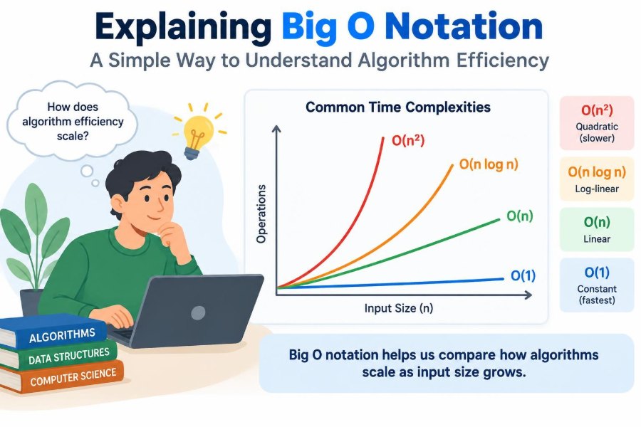
Big O notation gives developers a compact way to describe that change. It does not predict an exact number of seconds. Instead, it helps answer a more durable question: how does the amount of work grow as the input grows?
Once that question becomes familiar, algorithm choices become easier to explain, compare, and improve.
🧭 What Big O Notation Describes
Big O notation describes the growth rate of an algorithm’s resource use, usually its running time. The input size is commonly written as n.
If an algorithm is O(n), its work generally grows in proportion to the number of items. If it is O(n²), doubling the input can make the work roughly four times larger.
Big O can also describe memory use, network requests, or another limited resource. In everyday programming discussions, however, “Big O” usually means time complexity.
📦 Understanding the Input Size n
The symbol n is not always “the number of rows.” It represents the meaningful size of the problem being solved.
For an array search, n may be the number of elements. For sorting text, it may involve both the number of strings and their lengths. For a graph, it is often useful to track vertices and edges separately as V and E.
Choosing the right input measure matters. A complexity claim is only useful when readers know what is growing.
📈 Why Growth Matters More Than a Stopwatch
Two computers can run the same code at different speeds. A database cache, programming language, compiler, and machine workload can also change measured time.
Big O deliberately ignores those changing details. It compares the shape of growth, which is often the deciding factor once data becomes large.
An O(n²) routine might beat an O(n log n) routine on a tiny input because of simple implementation and low overhead. But the quadratic routine is more likely to become the bottleneck as the input expands.
🔭 Looking at Large Inputs
Big O is an asymptotic description: it focuses on behavior as input size becomes very large. This is why constant setup costs and small terms are often omitted.
That does not mean small inputs are irrelevant. A command-line tool that always processes ten records has different needs from a service that processes millions.
The practical lesson is to consider the expected input range. Big O provides a warning system for scaling, not a substitute for measuring real performance.
🧮 Ignoring Constants and Smaller Terms
Suppose an algorithm performs 3n + 20 operations in a simplified model. Its Big O is O(n), because the n term eventually dominates the fixed 20, and the factor 3 does not change the growth category.
Likewise, n² + 50n becomes O(n²). As n rises, the square term overwhelms the linear term.
This simplification is useful, but it has a limit. An O(n) process with an extremely expensive operation per item may still be slower than another O(n) process. Big O compares growth, not every cost.
⚖️ The Common Complexity Classes
The following classes are a useful first map. They describe broad patterns rather than a ranking that automatically decides every engineering choice.
| Notation | Typical pattern | Simple example |
|---|---|---|
| O(1) | Constant work | Read an array item by index |
| O(log n) | Repeatedly shrink the search space | Binary search |
| O(n) | Visit each item once | Find the largest value |
| O(n log n) | Divide and process across levels | Efficient comparison sorting |
| O(n²) | Compare many pairs | Simple nested-loop comparisons |
| O(2ⁿ) | Explore many include/exclude choices | Naive subset search |
| O(n!) | Try arrangements | Naive route permutation search |
Moving down this table is not merely a small slowdown. For sufficiently large inputs, the difference can be dramatic.
⚡ O(1): Constant-Time Work
O(1) means the amount of work does not grow with n. Accessing scores[42] in a normal array is a standard example: the program computes where that position is and retrieves it.
“Constant” does not mean instant. Reading a value, checking permissions, or making a network call may all take noticeable time. It means input size does not make that particular operation grow.
Hash table lookups are often described as O(1) on average, a qualification that matters when collisions or resizing are considered.
🔍 O(log n): Reducing the Search Space
Logarithmic algorithms make progress by discarding a large fraction of possibilities at each step. Binary search is the classic case.
To find a name in a sorted list, inspect the middle entry. If the target belongs later, ignore the first half; otherwise, ignore the second. Repeating this process quickly narrows the range.
Binary search requires sorted data and suitable access to the middle. Applying it blindly to an unsorted list will produce unreliable results.
🚶 O(n): One Pass Through Data
Linear time means work grows roughly with the number of items. To find the maximum temperature in a list, every value may need to be examined once.
largest = values[0]
for value in values:
    if value > largest:
        largest = value
One loop often suggests O(n), but the loop body matters. If it contains an operation whose cost grows with the input, the total may be more than linear.
🧩 O(n log n): Divide, Organize, Combine
Many practical sorting algorithms have O(n log n) average or worst-case behavior under their usual assumptions. The pattern often involves dividing data into smaller parts and doing a manageable amount of work at each level.
Imagine repeatedly splitting a pile of records in half. There are about log n splitting levels, while all records are processed across each level. That combination leads to n log n.
This class is often an excellent target when a task needs to organize a large collection rather than simply scan it.
🔲 O(n²): Work Across Pairs
Quadratic time commonly appears when every item is compared with many other items. For example, a straightforward duplicate check may compare each value against the values after it.
for i in range(n):
    for j in range(i + 1, n):
        compare(items[i], items[j])
The inner loop does not run exactly n times on every pass, but the total number of comparisons still grows proportionally to n². This is often acceptable for a few dozen items and risky for very large collections.
🌋 Exponential and Factorial Growth
O(2ⁿ) and O(n!) algorithms can become impractical surprisingly quickly because their work multiplies rapidly as input grows. They often arise in problems that try every subset, every decision sequence, or every ordering.
For a small puzzle instance, exhaustive search can be reasonable and wonderfully simple. For larger instances, developers usually seek pruning, dynamic programming, heuristics, or a different formulation.
A heuristic can produce a useful answer without checking every possibility, but it may not guarantee the mathematically optimal answer. That trade-off should be explicit.
🪜 Reading Loops Without Guessing
A loop is not automatically O(n), and nested loops are not automatically O(n²). Read what changes and how often.
- A loop that increments from 0 to
nis usually O(n). - A loop that doubles its counter each time is O(log n).
- Two loops that run one after another are usually added, such as O(n + n).
- A loop inside another loop usually multiplies their work when each runs independently.
Tracing a few input sizes can reveal the pattern. Then simplify the resulting expression using the dominant term.
➕ Sequential Steps Add Together
Consider a function that scans a list once to calculate a total, then scans it again to find the largest value. The simplified cost is O(n + n), which becomes O(n).
More generally, O(a + b) is appropriate when two collections have different sizes. If a function compares every user with every order, describing it as O(users × orders) is clearer than forcing both quantities into n.
Keeping separate variables prevents vague analysis and exposes where data relationships cause costs to grow.
✖️ Nested Steps Often Multiply
If an outer loop runs n times and an independent inner loop also runs n times for every outer iteration, the result is O(n × n), or O(n²).
But nesting alone is not proof. This code has nested loops but only O(n) total increments:
j = 0
for i in range(n):
    while j < n:
        j += 1
After the first pass, j has reached n; the inner loop does not restart. Follow state changes rather than relying on visual shape.
🔀 Best Case, Average Case, and Worst Case
Some algorithms take different amounts of work depending on the input. A linear search finds a target immediately if it is first, but may inspect every item if it is last or absent.
Worst-case complexity describes the upper bound for a given input size. It is valuable when predictable performance matters. Average-case complexity describes expected behavior under a stated model of typical inputs.
Do not assume “average” means ordinary real-world data without checking the assumptions. Input distributions, user behavior, and adversarial requests can differ from the model.
🛡️ Why Worst Cases Can Matter
A system exposed to untrusted input may need special attention to worst-case behavior. An attacker or accidental workload pattern can sometimes trigger slow paths repeatedly.
That does not mean every feature needs the most sophisticated algorithm. It means performance limits should be considered alongside correctness, reliability, and resource controls.
Timeouts, request-size limits, rate limits, and algorithmic improvements can all reduce operational risk. The right combination depends on the system.
🧠 Time Complexity Versus Space Complexity
Time complexity tracks work performed; space complexity tracks memory that grows while the algorithm runs. An algorithm may trade one for the other.
Checking duplicates with a nested comparison can use O(1) extra memory but take O(n²) time. Storing seen values in a hash set commonly reduces expected lookup work and uses O(n) additional memory.
Neither choice is automatically superior. On memory-constrained devices, extra storage may be costly. In a server handling large data, avoiding quadratic time may be more urgent.
🗂️ Data Structures Change the Story
Algorithm efficiency is inseparable from data structure choice. A list is convenient for ordered iteration, while a hash set is useful when fast membership checks are needed.
For example, repeatedly asking “have we already seen this identifier?” by scanning a list can lead to O(n²) total work. Using a set often makes the same overall task O(n) on average.
Still, data structures have costs: memory overhead, ordering behavior, update rules, and worst-case characteristics. Match the structure to the operations the program performs most often.
🧱 Sorting Can Be a Useful Investment
Sorting is not always wasted work. If a collection will be searched many times, sorting once in O(n log n) and then using O(log n) binary searches may be sensible.
By contrast, if only one search is needed, a single O(n) scan may be simpler and faster overall. The useful comparison includes preparation, number of queries, updates, and storage needs.
This is a general design habit: evaluate a sequence of operations, not just one operation in isolation.
🌳 Recursion and Recurrence Patterns
Recursive functions call themselves on smaller inputs. Their complexity depends on how many calls are made and how much work each call performs.
A function that reduces n by one each time is often O(n). One that splits into two branches can be far more expensive if both branches keep expanding.
For divide-and-conquer algorithms, ask three questions: how many subproblems are created, how large are they, and how much combination work happens at each level? Drawing a small call tree can make the answer visible.
🌐 Complexity Beyond a Single Machine
Big O does not capture every performance concern in a real application. Database queries, disk access, network latency, serialization, and lock contention can dominate a request’s elapsed time.
For example, an O(n) loop that makes one remote request per item may be much slower than an O(n²) in-memory calculation on a small dataset. The expensive resource is the network round trip, not just the loop count.
Use complexity analysis to understand computational growth, then profile the full system to find the actual bottleneck.
📏 Benchmarking Complements Big O
Benchmarks answer “how fast is this implementation on this workload and machine?” Big O answers “how will its work tend to grow?” Both are valuable, and neither replaces the other.
Useful benchmarks test realistic input sizes and shapes. A program can behave differently with already sorted data, repeated values, long strings, cache-friendly arrays, or data that exceeds available memory.
Measure after identifying a plausible problem. Randomly optimizing code without evidence can make it harder to maintain without improving the user experience.
🧪 A Practical Analysis Workflow
When reading unfamiliar code, use a repeatable process instead of trying to spot the answer instantly.
- Define the input sizes that can grow.
- Identify the main repeated operation, such as a comparison, lookup, or recursive call.
- Count how often that operation can happen in the relevant case.
- Combine sequential costs by addition and independent nested costs by multiplication.
- Keep the dominant growth term, then state relevant assumptions.
- Check whether data structure operations have their own nonconstant cost.
This process also makes code reviews more productive because it turns “this seems slow” into a specific, testable explanation.
🚫 Mistakes People Make With Big O
A common mistake is treating Big O as a precise runtime promise. O(n) does not tell you that a task will finish within a particular deadline.
Another is ignoring hidden work. Repeated string concatenation, list insertion at the front, copying arrays, or calling a search function inside a loop can change the true cost.
It is also easy to optimize a non-problem. Clear O(n²) code handling five items may be preferable to a complex solution whose maintenance cost outweighs its performance benefit.
🧰 Improving a Slow Algorithm Thoughtfully
Start by confirming what is slow and under which workload. A slow report might be caused by a repeated database query, not the local algorithm you first notice.
Then look for a structural improvement: avoid repeated scans, cache stable results, index data, replace pairwise comparisons with a set or map, or sort when repeated searches justify it.
Keep correctness checks in place. Faster code that changes ordering, misses duplicates, or handles edge cases incorrectly is not an improvement.
📝 Communicating Complexity Clearly
A good complexity note names the operation and the assumptions. “Expected O(n) time and O(n) extra space using a hash set” tells readers much more than simply “fast.”
When there are multiple inputs, preserve them: “O(V + E)” is informative for graph traversal because vertices and edges can grow independently.
Clear language also prevents false certainty. Say “average-case” or “worst-case” when that distinction affects the decision.
🎯 Choosing the Right Level of Efficiency
The best algorithm is not always the one with the smallest asymptotic notation. Readability, implementation time, available libraries, memory limits, and the expected scale all matter.
For an infrequent internal task with tiny inputs, straightforward code may be ideal. For a high-volume endpoint or recurring batch process, scaling behavior deserves earlier attention.
Good engineering is contextual: use Big O to see the likely growth problem, then choose a solution that fits the real constraints.
🏁 The Core Principle to Remember
Big O notation is a language for reasoning about growth. It helps you move beyond “this worked in my test” toward “what happens when the input becomes ten, a thousand, or a million times larger?”
Its most useful habits are simple: identify the growing input, count the repeated work, recognize whether work is added or multiplied, and account for data structures and assumptions.
Used this way, Big O is not a memorization contest. It is a practical tool for designing software that remains responsive as its workload changes.
Big O notation does not predict every second of runtime, but it reveals which algorithms are likely to keep working well as the problem grows. 💻📈🧠