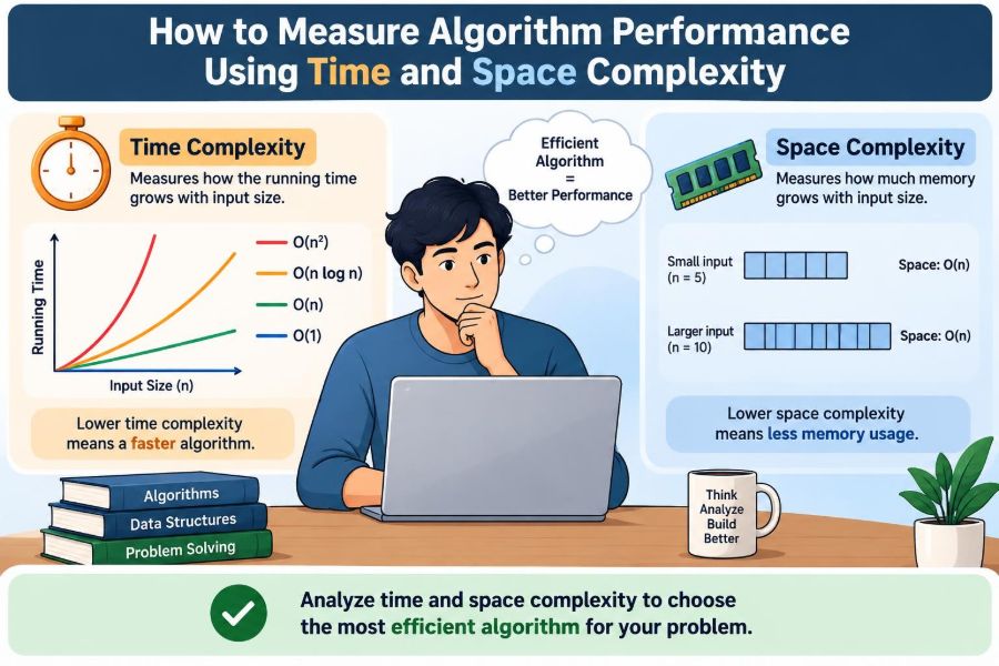

A program can work perfectly on ten records and still become frustratingly slow when it receives ten million. A search box may lag, a report may take minutes to load, or a phone app may close because it runs out of memory.
These failures are rarely about whether the code is “correct.” They are about how the amount of work and storage changes as the input grows.
Computer scientists use time complexity and space complexity to describe that growth. These ideas let us compare algorithms before deploying them and explain why two correct solutions can behave very differently in practice.
You do not need a stopwatch or a supercomputer to start analyzing performance. You need a clear model of the input, the operations being repeated, and the memory being retained.
🧭 What Algorithm Performance Really Means
An algorithm is a defined sequence of steps for solving a problem. Performance asks how demanding those steps become as the problem size increases.
Usually, we measure two resources: running time, meaning the computational work performed, and memory, meaning the storage needed while the algorithm runs. A performance analysis is not a promise that a program will take an exact number of seconds; it is a way to predict scaling behavior.
📏 Start by Defining the Input Size
Complexity uses a variable, conventionally n, for input size. For a list, n may be the number of items. For a string, it may be the number of characters. For a graph, it is often useful to track both vertices V and edges E.
Choose the measure that drives the work. Reading a file may depend on its bytes, while comparing all pairs of customers depends on the number of customers. An unclear definition of n produces an unclear analysis.
⏱️ Understanding Time Complexity
Time complexity describes how the number of fundamental operations grows with input size. A fundamental operation might be a comparison, arithmetic calculation, array access, or loop iteration.
Consider checking whether a name appears in an unsorted list. In the worst case, the algorithm examines every name. If the list doubles, the maximum number of checks roughly doubles too, which is linear growth.
🧠 Understanding Space Complexity
Space complexity describes how much memory an algorithm requires as input grows. The input itself occupies memory, but analysis often focuses on auxiliary space: additional memory created by the algorithm.
Finding the largest item in an array can use one variable for the current maximum, regardless of array length. Copying every item into a second array needs extra storage that grows with the array.
🔤 Why We Use Big O Notation
Big O notation expresses an upper-growth bound, commonly used to describe worst-case resource use. It ignores details such as processor speed, programming language overhead, and small fixed costs.
That simplification is useful because hardware changes, but growth patterns remain meaningful. Saying an operation is O(n²) warns that its work can rise roughly with the square of input size; this matters far more than a small constant difference when data becomes large.
🔍 Big O Is Not a Stopwatch
O(n) does not mean “fast,” and O(n²) does not mean “always unusable.” A small quadratic task can finish sooner than a linear task with expensive disk access or a large constant factor.
Big O compares long-term growth, not elapsed time on one machine. Use it alongside profiling and realistic tests when making production decisions.
➕ Simplifying Complexity Expressions
When reporting Big O, keep the term that grows fastest and drop constant multipliers. For example, 3n + 20 becomes O(n), while n² + 8n becomes O(n²).
This does not claim the discarded work disappears. It means that for sufficiently large inputs, the dominant term determines the overall growth class. During optimization of small, fixed workloads, those constants can still matter.
🟢 Constant Time: O(1)
An operation is O(1) if its cost stays bounded as n changes. Accessing an array element by a valid index, such as scores[4], is the standard example.
Constant time does not mean zero time. It means accessing item 4 does not require scanning the preceding items. Hash table lookup is often treated as average-case constant time, although collisions and implementation details can affect individual operations.
📈 Linear Time: O(n)
A single pass through a collection is usually O(n). Summing all invoice amounts, checking every character for a forbidden symbol, and finding the largest number are common examples.
max = items[0]
for each item in items:
    if item > max:
        max = item
The loop runs once per item, while the work inside remains bounded. Therefore the running time grows linearly.
🪜 Logarithmic Time: O(log n)
Logarithmic algorithms repeatedly shrink the remaining problem by a fixed factor. Binary search illustrates this: in a sorted list, compare with the middle item, then discard approximately half the possible locations.
Binary search requires sorted data and random access to the middle position. It is not a universal replacement for scanning; maintaining a sorted collection can itself have a cost.
🌿 Linearithmic Time: O(n log n)
Many efficient comparison sorting algorithms run in O(n log n) time in their typical or guaranteed cases. Merge sort divides the data into halves, then combines sorted halves; each level handles all items, and there are logarithmically many levels.
This growth is usually far more manageable than quadratic sorting for large collections. The exact trade-offs differ: merge sort commonly uses extra memory, while other sorting methods may use less auxiliary space but have different worst cases.
🧱 Quadratic Time: O(n²)
Nested loops are often quadratic when each loop runs through the same n items. For example, comparing every product with every other product creates roughly n × n comparisons.
A nested loop is not automatically quadratic. If the inner loop runs a fixed ten times, the total is still O(n). Count how iterations depend on input size rather than judging by indentation alone.
🚨 Exponential and Factorial Growth
O(2ⁿ) and O(n!) algorithms can become impractical surprisingly quickly because their work multiplies dramatically with each added input item. Trying every subset is a common exponential pattern; trying every ordering is a common factorial pattern.
Such algorithms are sometimes necessary for small instances or exact solutions. In larger cases, developers often seek pruning, dynamic programming, approximation, or a different formulation of the problem.
🗂️ A Quick Growth-Rate Reference
| Complexity | Typical pattern | Example use |
|---|---|---|
O(1) |
Fixed work | Array index access |
O(log n) |
Repeated halving | Binary search |
O(n) |
One full pass | Finding a maximum |
O(n log n) |
Divide and combine | Efficient comparison sorting |
O(n²) |
Many pairs | Comparing all pairs |
The table is a guide to growth, not a ranking that removes context. Inputs, constants, hardware behavior, and required results still shape the best choice.
🔁 Count Sequential Blocks by Adding Them
If one block scans a list and a later block scans it again, the work is O(n) + O(n), which simplifies to O(n). The blocks happen one after another, so their costs add.
For a scan followed by a nested pair comparison, the result is O(n + n²), or O(n²). The slower-growing first pass remains real work, but it does not dominate at large sizes.
🪆 Count Nested Work by Multiplying It
When an inner operation runs for every iteration of an outer loop, multiply their iteration counts. An outer loop of n and inner loop of m gives O(nm).
This distinction matters for rectangular data. Comparing every row in one dataset to every row in another may be O(ab), not necessarily O(n²), because the datasets can have different sizes.
🔀 Analyze Branches and Worst Cases
An if statement does not add both branch costs during a single execution. For worst-case Big O, analyze the most expensive branch that can occur.
Suppose a function returns immediately if a cached result exists but otherwise sorts n items. Its best case may be O(1); its worst case is driven by sorting. Both descriptions can be useful if you state the condition clearly.
🎯 Best, Average, and Worst Case
Best-case complexity describes favorable inputs, worst-case complexity describes the highest work within the model, and average-case complexity describes expected work under stated assumptions about inputs.
Worst case is popular because it gives a bound, but it is not always the most useful operational measure. A service handling mostly successful hash lookups may care strongly about average behavior, while a real-time task may need predictable worst-case latency.
🧪 Measure Real Programs with Benchmarks
Asymptotic analysis answers “how will this scale?” Benchmarking answers “how does this implementation behave here?” Measure representative input sizes, repeat runs, and avoid treating one noisy timing as a conclusion.
- Use realistic data shapes, not only random values.
- Separate setup work from the operation being compared.
- Check memory use as well as elapsed time.
- Test growth across several input sizes rather than one size.
Warm-up behavior, caching, input/output, garbage collection, and operating-system activity can influence timings. These are reasons to interpret measurements carefully, not reasons to avoid measuring.
🧰 Use a Profiler to Find the Actual Bottleneck
A profiler records where a program spends time or allocates memory. It can reveal that a supposedly expensive algorithm is not the slowest part of the application; perhaps repeated database requests, parsing, or rendering dominates instead.
Profile before making complex changes. Improving a function that consumes little time may make code harder to maintain without producing a noticeable user benefit.
💾 Recognize Common Space Patterns
Variables holding a few counters, indexes, or references generally use O(1) auxiliary space. An output array containing one transformed value per input item uses O(n) space.
For a two-dimensional grid with r rows and c columns, storing all cells requires O(rc). A graph representation may need space proportional to vertices plus edges, often written O(V + E).
📚 Recursion Uses Hidden Stack Space
Every recursive call usually creates a stack frame containing local state and a return location. A recursive function that descends through n items can therefore use O(n) call-stack space, even if it creates no array.
Balanced divide-and-conquer recursion may have depth O(log n). Very deep recursion can also hit language or environment stack limits, so an iterative approach may be safer when depth is unpredictable.
⚖️ Time-Space Trade-Offs
Algorithms often save time by storing extra information. A hash set can make repeated membership checks fast on average, but it consumes memory. A cache can avoid recomputing results, but cached entries must be bounded and invalidated correctly.
Conversely, recalculating values can reduce memory use at the cost of extra CPU work. Neither direction is automatically better; the right decision depends on memory limits, response-time goals, data size, and access patterns.
🧩 Data Structures Change the Analysis
The same task can have different complexity depending on the data structure. Checking whether a value exists in an unsorted array takes a linear scan in the general case, while lookup in a well-designed hash set is commonly average O(1).
A sorted array supports binary search, but inserting a new item may require shifting many elements. A linked structure can make some insertions inexpensive once the location is known, but locating that position may still require traversal. Always analyze the full workload, not one attractive operation.
🛑 Avoid Premature Optimization
Replacing clear code with a sophisticated algorithm before identifying a real constraint can introduce bugs and obscure the program’s purpose. For small inputs, a straightforward O(n²) solution may be perfectly appropriate and easier to verify.
Do not ignore scalability either. If input size is unbounded or a routine runs frequently, estimate its growth early. The practical approach is to choose a clear baseline, measure it, and optimize where evidence and constraints justify the effort.
🧯 Common Complexity Analysis Mistakes
- Ignoring library calls: sorting, copying, string concatenation, and membership tests may do substantial work internally.
- Assuming nested loops always mean O(n²): inspect each loop’s actual bounds.
- Forgetting output space: a result with
nitems inherently needs room somewhere. - Calling average-case behavior guaranteed: state the assumptions behind the claim.
- Optimizing only CPU time: memory pressure can cause equally serious slowdowns or failures.
Writing the input size and the key repeated operation beside a code fragment prevents many of these errors.
📝 A Repeatable Method for Analyzing Code
- Define the input variables, such as
n,V, andE. - Identify the operation or block repeated most often.
- Count sequential blocks by addition and nested blocks by multiplication.
- Consider branches, recursion depth, and calls to other algorithms.
- Simplify the expression to its dominant growth term.
- Analyze extra memory separately from the input and required output.
- Validate important conclusions with profiling and representative benchmarks.
This method is more reliable than memorizing labels because it connects the notation directly to the code’s behavior.
🏁 The Core Principle: Predict Growth, Then Choose Wisely
Time and space complexity are tools for reasoning, not scores for judging code in isolation. They reveal how an approach reacts when the workload grows and where a design may cross a practical limit.
Start with the problem’s constraints: expected input size, response-time needs, available memory, frequency of execution, and the cost of complexity in the code itself. Then compare plausible algorithms and data structures using both asymptotic analysis and real measurements.
The best algorithm is the one whose time, memory use, and implementation complexity fit the actual problem—not simply the one with the smallest-looking Big O label. With that mindset, performance analysis becomes a practical design habit rather than a collection of symbols. 💻📊🧠