If we look at our top down methodology from last week, we’ll see that we have enumerated through all of the permutations of paths — that is to say, we have brute-forced our way to determine every single route that our traveling salesman could take.

The brute-force approach to solving TSP.

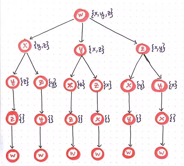
This methodology isn’t particularly elegant, is kind of messy, and, as we have already determined, will simply never scale as our input size grows. But ignoring all of those issues for a moment, let’s just take a look at this “tree” of recursive function calls once again.

Rethinking the brute-force approach by identifying the simplest problem, or function call.

On second glance, we’ll notice that there is something interesting going on here: we’re starting with the more complex function call initially, and then, from within that, we are invoking three recursive function calls from within it. Each of those three recursive function calls spins off two more recursive calls of its own, which creates the third level of this function call “tree”. This is, of course, keeping in tune with our working definition of a top down approach: starting with the largest problem first, and breaking it down into its smallest parts. But, now that we can see the smallest parts more obviously, we can change our approach from a top down method to a bottom up method.

We’ll recall that a bottom up dynamic programming approach starts with the smallest possible subproblems, figures out a solution to them, and then slowly builds itself up to solve the larger, more complicated subproblem. In the context of our “function call tree”, the smallest possible subproblem are the smallest possible function calls. We’ll see that the smallest function calls are the simplest ones — the ones that have no recursive calls within them. In our case, these are the function calls at the very bottom of our “function call tree”, which lead back to our starting node, node w, which is the city that our traveling salesman is “starting” from, and will inevitably have to “end” up at.

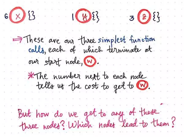
Now that we’ve identified the smallest possible subproblems, we can turn TSP on its head. We’ll flip our top down approach to this problem and, instead, use a bottom up approach here. Let’s start with our three simplest function calls.

Flipping TSP on its head, part 1.

We’ll see that each of these calls connects back to w, as we would expect. Recall that we’re using a list notation to keep track of the nodes that we can navigate to. Since we’re dealing with the smallest possible subproblem(s), there is nowhere that we can navigate to from these nodes; instead, all we can do is go back to our starting node, w. This is why each of the lists for these three subproblems is empty ({}).

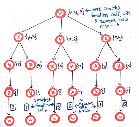
However, we do need to keep track of cost and distance here, since inevitably, we’re still going to have to find the shortest path for our traveling salesman, regardless of whether we’re using a top down or bottom up approach. Thus, we’re going to have to keep track of the distance between nodes as we build up our “bottom up” tree. In the image above, we’ll see that we have the values 6, 1, and 3 next to nodes x, y, and z, respectively. These number represent the distance to get from each node back to the origin node, w.

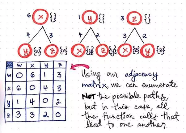
When we first tried to solve TSP, we used an adjacency matrix to help us keep track of the distances between nodes in our graph. We’ll lean on our adjacency matrix in this approach yet again.

However, in our bottom up approach, we’ll use it to enumerate all the function calls that lead to one another. This is strikingly different than our top down approach, when we were using our adjacency matrix to help us enumerate all the possible paths. In our bottom up approach, we’re trying to be a bit more elegant about how we do things, so we’re aiming to not enumerate more than we need to! This will make more sense as we go on, but it’s important to note the difference between enumerating paths versus enumerating function calls.

So, what would the second level of our function call “tree” look like? Well, the question that we’re trying to answer for each of our smallest possible subproblems here is this:

If we are at the simplest possible version of this function call and cannot call anything recursively from within this function, what other function could possibly call this one?

Flipping TSP on its head, part 2.

Another way of thinking about it is in terms of nodes. Ultimately, we’re trying to determine which possible nodes would allow us to get to the node that we’re looking at. So, in the case of node x, the only way to get to node x would potentially be node y or node z. Remember that we’re using a bottom up approach here, so we’re almost retracing our steps backwards, starting at the end, and working our way back through the circle.

Notice, again, that we’re keeping track of the cost/distance from each of these nodes to the next. We’re going to need them pretty soon!

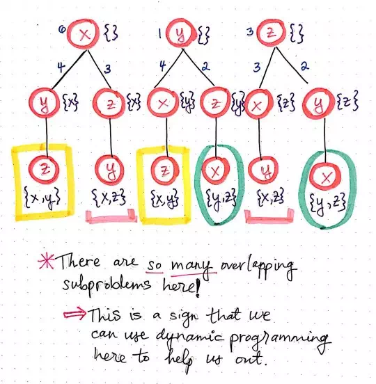
Again, we can expand this function call “tree” a bit more to add another level. Remember, we’re trying to answer the question: what other function could possibly call this function that we cannot expand any further?

Flipping TSP on its head, part 3.

In the drawing depicted here, we’ll see what this actually looks like in practice. For example, looking at the leftmost branch of this function call “tree”, we’ll notice that the only possible function call that will allow us to get to an empty node x is from either node y or node z, where the set contains only a possible “next” node of x, like so: {x}. For both node y and z in the leftmost subtree, we’ll see that the only possible way to get to y is from node z, when the set contains both x and y (or {x, y}). Similarly, the only possible way to get to z is from node y, when the set contains both x and z (or {x, z}).

This is a visualization exemplifies what we mean when we say that we are enumerating function calls rather than enumerating potential paths. As we continue to determine all the possible function calls that allow us to call other functions from within them, something starts to become very obvious: we have some overlapping subproblems here!

We’ll notice that there are two function calls that are instances of z when its set contains both x and y (or {x, y}), which is highlighted in yellow. Similarly, there are two function calls that are instances of y when its set contains both xand z (or {x, z}), highlighted in pink. Finally, we’ll see two function calls that are instances of x when its set contains both y and z (or {y, z}), highlighted in green.

Dynamic programming is all about identifying repeated work and being smarter and more efficient with our approach so that we don’t actually have to repeat ourselves! So, let’s cut out this repetition and use some dynamic programming to make things a little better for our traveling salesman.