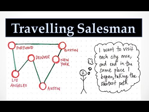
Now that we’ve identified our overlapping and recurring subproblems, there’s only one thing left to do: eliminate the repetition, of course!

Flipping TSP on its head, part 4.

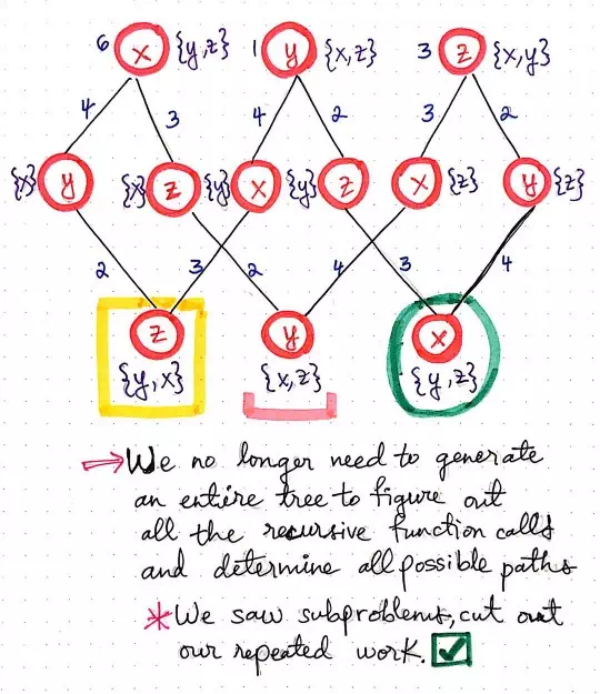
Using our function call “tree”, we can rearrange some of our function calls so that we’re not actually repeating ourselves in level three of this tree.

We can do this by cutting down our repeated subproblems so that they only show up once. Then, we’ll reconfigure the bottom level of our tree so that it is still accurate, but also that we each function call show up once, not twice.

Now it starts to become apparent how the bottom up approach is different than our top down method from before.

We’ll see that we no longer need to do the work of generating that entire bottom level of our function call “tree” in order to figure out all o the recursive function calls. Nor do we need to determine all the possible paths that our traveling salesman could take by using brute force. Instead, we’re enumerating through function calls, finding the repeated ones, and condensing our “tree” of function calls as we continue to build it.

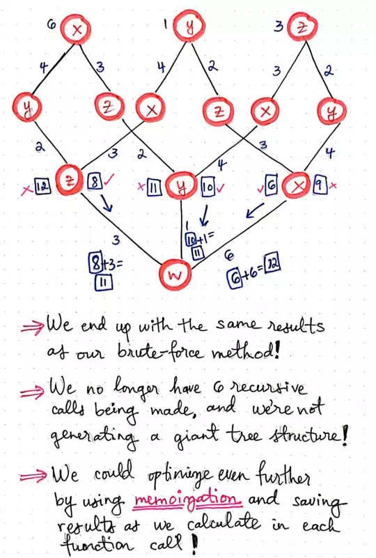
Once we’ve eliminated the repeated subproblems, we can do the work of actually finding the shortest path. Remember that we will need to use our adjacency matrix to figure out the distance between one node to another. But, we’ll also notice that we’re not having to repeat ourselves nearly as much because we won’t see the same numbers appear too many times as we sum them up.

In the illustration shown below, each of the function calls that allow our salesman to traverse from one node to another has a number (the cost or distance) associated with it. As we continue down this tree, we’ll sum up the cost of each set of function calls. For example, if we choose the function calls that lead from w <- x <- y <- z, we’ll sum up the cost between these nodes, which amounts to 6 + 4 + 2 = 12.

Flipping TSP on its head, part 5.

When we get down to the third level of our function call “tree”, we’ll see that we have two numbers that we can choose from. Recall that we had a similar scenario happen to us in our top down approach last week: we had two different paths with two different costs/distances to choose from. We ended up choosing the smaller of the two cost, since we’re trying to find the shortest path for our salesman. In this case, we have two different function calls, with two different costs/distances to choose from. Again, we’ll choose the smaller of the two costs, since we’re still trying to find the shortest path here, too!

Eventually, as we continue sum the distances/costs, we’ll see that we ended up witht he exact same results as our brute-force method from last week. The shortest cost for our traveling salesman is going to be 11, and there are two possible paths that would allow for them to achieve that lowest cost. However, using the bottom up approach, we’ve optimized our TSP algorithm, since we no longer have six recursive calls being made in this method. Furthermore, we’re also not generating as big of a tree structure! If we think back to when we were first introduced to dynamic programming, we’ll recall that we could also use memoization and save the results of our function calls as we calculate them, optimizing our solution even further.

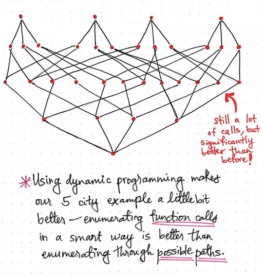
Using dynamic programming makes our 5 city example a little faster.

Okay, so we started down this path in an effort to take the next step in the adage of “Make it work, make it right, make it fast.”

We have arguably made our workable solution much better, and certainly more elegant, and far less repetitive. The illustration shown here exemplifies how the bottom up DP approach would scale for a traveling salesman problem where the salesman has to visit five cities instead of four. We’ll see that we’re still making a lot of calls, but our function call “tree” is a bit slimmer and significantly better than before.

By using dynamic programming, we’ve made our solution for the traveling salesman problem just a little bit better by choosing to smartly enumerate function calls rather than brute-force our way through every single possible path that our salesman could take.

The only question we have to answer now is, of course, how does the runtime of this method compare to our ugly factorial, O(n!) runtime from earlier?

Well, as it turns out, the bottom up approach that we’ve been exploring here is really the foundations of something called the Held-Karp algorithm, which is also often referred to as the Bellman-Held-Karp algorithm. This algorithm was derived in 1962, by both Michael Held and Richard M. Karp as well as Richard Bellman, who was working independently on his own related research at the time.

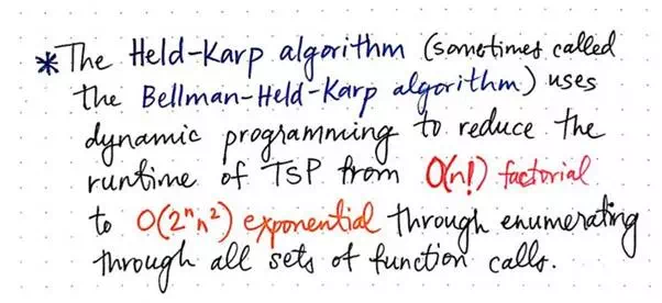
The Held-Karp algorithm uses dynamic programming to approach TSP.

The Held-Karp algorithm actually proposed the bottom up dynamic programming approach as a solution to improving the brute-force method of solving the traveling salesman problem. Bellman, Held, and Karp’s algorithm was determined to run in exponential time, since it still does a bulk of the work of enumerating through all the potential sets of function calls that are possible. The exponential runtime of the Held-Karp algorithm is still not perfect — it’s far from it, in fact! But, it’s not as ugly as a factorial algorithm, and it’s still an improvement.