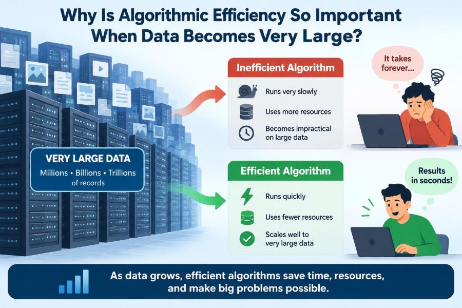

A search box that responds instantly feels ordinary—until it does not. A slow result page, a frozen spreadsheet, or an app that times out during checkout makes the hidden work of computing suddenly visible.
Often, the machine has not become weaker and the program has not changed very much. What changed is the amount of data: a customer list became a customer history, a few photos became a library, or thousands of events became millions.
This is where algorithmic efficiency matters. An algorithm is a repeatable method for solving a problem, and its efficiency describes how its need for time or memory grows as the problem grows.
For small inputs, many approaches appear equally good. At large scale, tiny differences in growth can turn a useful program into one that is expensive, delayed, or unable to finish at all.
🧭 The Meaning of Algorithmic Efficiency
Algorithmic efficiency is not simply “fast code.” It concerns the resources an algorithm consumes, most commonly running time and memory, as input size increases.
Suppose two programs both find a matching record. One checks records one by one; another uses a prepared index. Their performance may look similar with ten records, but their behavior can diverge sharply with ten million.
Efficiency asks a scalable question: if the input becomes larger, what happens to the amount of work?
📏 Input Size Is the Real Variable
Computer scientists usually call input size n. Depending on the task, n could mean the number of rows in a table, characters in a document, pixels in an image, graph connections, or requests arriving at a service.
“Large” is relative. A million short identifiers may be manageable in memory, while a million high-resolution images may not be. The useful question is not whether a number sounds large, but whether the algorithm’s growth matches the available resources and response-time requirement.
📈 Why Growth Rate Beats a Single Timing Test
Testing a program once and reporting that it takes two seconds is incomplete. The result depends on the machine, current workload, programming language, input shape, and test size.
Growth rate is more durable. If doubling the input roughly doubles the work, the algorithm behaves very differently from one where doubling the input makes the work roughly four times larger.
Timing measurements still matter in production. But growth analysis helps explain what timings are likely to do before an expensive failure arrives.
🔢 Big O Gives a Useful Growth Vocabulary
Big O notation describes an upper-bound-style category for how work grows with input size. It deliberately ignores fixed constants and smaller terms so that the dominant long-term pattern is easier to see.
An algorithm described as O(n) grows linearly: processing twice as much data requires roughly twice as much work. An O(n²) algorithm grows quadratically: doubling the data can require roughly four times as much work.
Big O does not predict an exact runtime. It is a model for comparing scaling behavior, not a stopwatch reading.
🧮 Common Complexity Classes at a Glance
| Complexity | Typical idea | Scaling intuition |
|---|---|---|
O(1) |
Direct array access | Work stays roughly constant |
O(log n) |
Binary search | Problem is repeatedly halved |
O(n) |
Scan every item once | Work grows with items |
O(n log n) |
Efficient comparison sorting | Usually practical for large collections |
O(n²) |
Compare every pair | Growth becomes costly quickly |
O(2ⁿ) |
Try many combinations | Becomes impractical very rapidly |
These labels are guides, not verdicts. An O(n²) method may be perfectly sensible for a small fixed list, while an O(n log n) method may carry overhead that is not worthwhile for tiny inputs.
🔍 Linear Search Reveals the Scaling Problem
Imagine looking for a name in an unsorted contact list. A linear search checks entries from the beginning until it finds the target or reaches the end.
In the worst case, it inspects all n entries, so it is O(n). This is often a reasonable choice when searches are rare, the data changes constantly, or the collection is small.
The trouble begins when the same large collection is searched repeatedly. Repeating a full scan for every request means doing large amounts of nearly identical work again and again.
✂️ Binary Search Uses Order as Information
Binary search works on sorted data. Rather than checking one item at a time, it examines the middle item and discards the half that cannot contain the target.
Each comparison cuts the remaining search region approximately in half. That gives binary search O(log n) time, an enormous advantage for large, static, sorted collections.
Its limitation is equally important: keeping data sorted has a cost, and binary search is not directly useful when the data structure cannot efficiently reach the middle or when the ordering does not match the question.
🗂️ Indexes Trade Preparation for Fast Retrieval
A database index is much like the index at the back of a book. It stores an organized route to records so the database need not inspect every row for many common queries.
Indexes can accelerate reads dramatically, but they are not free. They occupy storage and must be updated when indexed data changes. Too many indexes can slow inserts, updates, and deletes.
The lesson is broader than databases: doing structured work once can avoid repeating expensive work later.
🔁 Nested Loops Can Create Quadratic Work
A nested loop is not automatically bad. But when an outer loop visits every item and an inner loop also visits every item, the total number of checks can approach n².
Consider checking whether any two user IDs in a list are equal by comparing every possible pair. With a small list, this is easy to write and fast enough. With a very large list, the pair count grows far faster than the list itself.
A hash-based set can often detect duplicates in expected linear time, showing how choosing the right data structure can change the algorithm’s growth.
🧩 Data Structures Shape the Cost of Operations
An algorithm does not operate in a vacuum. Its actual operations depend on the data structure used to store information.
- An array supports fast access by position but inserting near the beginning may require shifting items.
- A hash table often supports fast expected lookup by key but does not naturally keep keys sorted.
- A balanced tree can support ordered lookup and range queries efficiently.
- A queue supports processing in arrival order without repeatedly moving all elements.
Choosing a structure should start with the operations the application performs most often, not with which structure feels most familiar.
🧠 Time Efficiency Is Only Half the Story
A fast algorithm may consume substantial memory. For example, caching stores previously computed results so future requests can return quickly, but the cache must occupy memory and be managed.
Memory pressure can make a supposedly fast program slow. If the system runs out of available RAM, it may move data to much slower storage or terminate a process.
Good design considers both time complexity and space complexity: how much extra memory grows with input size.
💾 When Data No Longer Fits in Memory
Many classroom examples assume all input fits comfortably in RAM. Real datasets may live on disks, across database servers, or in cloud object storage, where moving data can dominate the total cost.
Sequential reading is usually friendlier to storage than repeatedly jumping to scattered locations. Algorithms designed for external data often reduce disk reads, process data in chunks, or sort and merge streams instead of loading everything at once.
At this point, an algorithm with an attractive CPU complexity can still perform poorly if it causes excessive input/output work.
🌐 Network Transfers Add Another Bottleneck
Distributed systems face a related problem: sending data between machines is much slower and less predictable than using data already in local memory.
A design that requires every server to exchange large intermediate results may be limited by network bandwidth and coordination delays rather than processor speed. Moving computation closer to data can be better than moving all data to computation.
This is why scalable systems pay close attention to data partitioning, batching, and minimizing round trips.
⏱️ Latency and Throughput Measure Different Things
Latency is the time one operation takes from start to finish. Throughput is the amount of work a system completes over a period, such as requests handled per second.
An algorithm may offer good average throughput by processing jobs in batches while giving an individual user a longer wait. Another may prioritize low latency but consume more resources per request.
The appropriate trade-off depends on the task. A background report can wait; an interactive autocomplete field cannot feel consistently delayed.
📊 Average Case, Worst Case, and Real Inputs
Complexity analysis often distinguishes worst-case, average-case, and best-case behavior. A linear search finds an item immediately in its best case but may inspect every item in its worst case.
Average-case claims rely on assumptions about typical input distributions. Those assumptions may not hold for real user behavior, skewed data, or inputs chosen deliberately to trigger bad behavior.
For systems with reliability requirements, examining worst-case behavior and tail latency—the slowest requests—can matter more than celebrating a fast average.
🛡️ Poor Complexity Can Become a Security Risk
Some inputs make particular algorithms perform far more work than usual. If an attacker can repeatedly submit such inputs, they may consume CPU time, memory, or database capacity and reduce service availability.
Examples include patterns that cause inefficient text matching, enormous nested inputs, or key distributions that stress poorly designed hash-table behavior. The exact risk depends on the language, libraries, and safeguards in use.
Input limits, timeouts, resource quotas, and algorithms with reliable worst-case behavior are practical defensive tools.
🧹 Sorting Often Makes Later Work Cheaper
Sorting costs work upfront, commonly O(n log n) for efficient comparison-based methods. That cost can pay off when ordered data enables faster searching, grouping, deduplication, or merging.
For example, two sorted lists can often be compared in one forward pass instead of comparing every item in one list against every item in the other. The order creates a useful structure.
However, sorting solely out of habit is wasteful when the task needs only a single pass, such as finding a maximum value.
🧬 Hashing Is Fast but Not Magic
Hashing converts a key into a location or bucket, enabling expected constant-time lookup in many hash table implementations. It is excellent for membership tests, key-value mappings, and duplicate detection.
Collisions occur when distinct keys map to the same location. Well-designed implementations handle collisions, but performance can deteriorate in unfavorable cases or when tables are poorly sized.
Hash tables also generally do not provide sorted traversal or efficient “find every key between A and B” queries. Fast lookup is not the same as being right for every query.
🧱 Constant Factors Still Matter
Big O ignores constant factors, but computers do not. An O(n) routine that allocates many objects, makes remote calls, or performs costly conversions can be slower than a higher-complexity alternative at the sizes an application actually uses.
Memory layout, cache behavior, language runtime overhead, and implementation quality all affect observed performance. This is why developers should combine complexity reasoning with profiling.
The sensible order is: avoid bad growth first, then measure and improve genuine bottlenecks.
🧪 Benchmarking Needs Representative Data
A benchmark based only on neat, tiny test data can hide the exact behavior that matters in production. Realistic tests should include plausible data volumes, request patterns, and difficult cases.
For a search feature, test misses as well as hits. For a database query, test uneven distributions and realistic concurrent load. For a parser, test large and deeply nested valid inputs within safe limits.
Measurements should be repeated because background activity and runtime warm-up can distort one-off results.
🔬 Profiling Finds the Work You Actually Do
Profiling records where an application spends time, allocates memory, or waits on input/output. It replaces guesses such as “the loop must be slow” with evidence.
A slow page may be caused by an inefficient algorithm, but it may also be waiting on a database query, serializing a huge response, or making repeated network calls. Optimizing the wrong part adds complexity without solving the user’s problem.
Use profiling after forming a hypothesis, and verify the improvement with a repeatable measurement.
🪜 Precomputation Changes the Cost Schedule
Precomputation performs work before it is immediately needed. Search indexes, lookup tables, materialized summaries, and compiled assets all use this idea.
It is valuable when many later requests reuse the prepared result. A route-planning system, for instance, may benefit from precomputed information for a stable map, while highly volatile data can make the maintenance cost too high.
The trade-off is between preparation time, memory or storage, freshness of results, and response speed.
🧊 Caching Helps Repeated Questions
A cache keeps a result close at hand so the system can avoid recalculating or re-fetching it. It can greatly reduce load when many people request the same content or calculation.
Caches introduce difficult questions: When does cached data expire? What happens after the underlying data changes? How much memory is available? A stale price, permission, or inventory count may be unacceptable.
Cache only when reuse is likely and define correctness rules before treating it as a performance cure.
🪟 Streaming Avoids Holding Everything at Once
Streaming processes data incrementally rather than collecting the full dataset before starting. A log processor can read one event at a time, update counts, and discard the event when it is no longer needed.
This can reduce memory from growing with the whole dataset to using a bounded working set. It also allows useful results to appear before a very large input has fully arrived.
Streaming is harder when the task requires global knowledge, such as exact sorting of all items or comparing a record with every future record.
🧭 Approximation Can Be the Right Engineering Choice
Some problems are expensive to solve exactly at huge scale. In appropriate contexts, approximate algorithms offer a controlled trade-off: use less time or memory while accepting a bounded or probabilistic loss of precision.
A system estimating broad trends may not need to retain every individual event forever. By contrast, accounting totals, access-control decisions, and safety-critical calculations usually require carefully defined exactness.
Approximation is not a shortcut for carelessness. Its error behavior must be understood, communicated, and suitable for the decision being made.
⚖️ Read-Heavy and Write-Heavy Workloads Need Different Choices
An index, cache, or precomputed summary often benefits systems that are read frequently. But every write may then require extra maintenance to keep those structures accurate.
A product catalog with many searches and occasional updates may justify several indexes. A rapidly changing event stream may favor simpler writes and later batch analysis instead.
There is no universally fastest design. Efficient systems match their costs to the workload they actually have.
🚫 Premature Optimization Creates Its Own Cost
Efficiency matters, but complex optimization added before a need is understood can make code harder to test, explain, and modify. It may also introduce subtle correctness bugs.
Do not interpret this as permission to ignore clearly poor algorithms. Avoiding an accidental O(n²) operation in a growing request path is basic design, not premature optimization.
A practical approach is to choose a sound algorithmic baseline, set performance expectations, measure realistic behavior, and optimize where evidence points.
🧰 A Practical Efficiency Checklist
- Identify the input size that will grow: records, users, files, requests, or relationships.
- List the operations performed most often and estimate their time and memory costs.
- Look for repeated scans, nested comparisons, unnecessary sorting, and repeated remote calls.
- Choose data structures that support the dominant operations.
- Measure with representative data, then profile before changing code.
- Account for storage, network transfer, concurrency, and correctness—not CPU time alone.
This checklist keeps performance work connected to a real system rather than to complexity notation alone.
🎯 The Core Principle at Large Scale
Data growth magnifies algorithmic choices. An inefficient step hidden inside a request, loop, or query may be harmless at first, then become the main reason a system feels slow or costs more to operate.
Efficient design means selecting methods whose growth fits the expected workload, recognizing trade-offs in memory and maintenance, and validating assumptions with measurement. It does not mean pursuing the mathematically fastest method at every cost.
The most durable question is simple: as this data grows, will this operation still be reasonable? Asking it early leads to clearer designs and fewer scaling surprises.
Algorithmic efficiency matters because large data turns growth patterns into real limits on speed, cost, reliability, and user experience. Learn the pattern, choose the trade-off deliberately, and measure the result. 💻📈🧠