
Some computational problems look simple at first but become extremely expensive as their size increases. A program may repeatedly solve the same smaller problems thousands, millions, or even billions of times without realizing it. 💻
Dynamic programming, often abbreviated as DP, is a powerful problem-solving technique designed to eliminate this waste.
The central idea is surprisingly straightforward:
Solve a smaller problem once, save the answer, and reuse it whenever the same result is needed again.
By storing previously calculated results, dynamic programming can transform certain algorithms from painfully slow solutions into highly efficient ones. 🚀
It is widely used in computer science, mathematics, artificial intelligence, operations research, economics, bioinformatics, route planning, resource allocation, and many other fields.
But dynamic programming is more than simply “remembering answers.” It works particularly well when a problem has specific mathematical properties that allow a large problem to be constructed from smaller, overlapping subproblems.
Understanding how DP works can dramatically improve the way programmers approach optimization and algorithmic challenges.
🧩 What Is Dynamic Programming?
Dynamic programming is an algorithmic technique for solving a complex problem by dividing it into smaller subproblems, solving each important subproblem once, and storing its result.
When the same subproblem appears again, the algorithm retrieves the stored answer rather than recalculating it.
This approach is useful when a problem has two important characteristics:
🔁 1. Overlapping Subproblems
The same smaller problems appear repeatedly during computation.
Instead of solving them again and again, dynamic programming stores their results.
🏗️ 2. Optimal Substructure
The optimal solution to the larger problem can be constructed from optimal solutions to smaller versions of the problem.
When both characteristics are present, dynamic programming can often produce dramatic improvements in performance.
🔢 A Simple Example: Fibonacci Numbers
The Fibonacci sequence provides one of the easiest ways to understand dynamic programming.
The sequence begins:
0, 1, 1, 2, 3, 5, 8, 13, 21, 34…
Each number is the sum of the previous two.
Mathematically:
F(n) = F(n – 1) + F(n – 2)
with:
F(0) = 0
F(1) = 1
A straightforward recursive implementation might calculate Fibonacci numbers like this:
fib(n):
    if n <= 1:
        return n

    return fib(n - 1) + fib(n - 2)
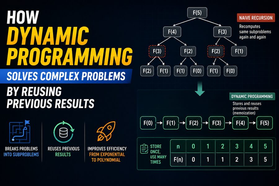
This code looks elegant, but it performs a huge amount of unnecessary work.
To calculate fib(5), the program calculates:
fib(5)
├── fib(4)
│   ├── fib(3)
│   │   ├── fib(2)
│   │   └── fib(1)
│   └── fib(2)
└── fib(3)
    ├── fib(2)
    └── fib(1)
Notice that fib(3) and fib(2) are calculated multiple times. 🔄
For larger values of n, this duplication becomes enormous.
🐌 Why Naive Recursion Becomes Slow
The simple recursive Fibonacci algorithm has approximately exponential time complexity.
Its running time grows roughly like:
O(2ⁿ)
That means increasing the input by only a small amount can dramatically increase the amount of computation.
For example, calculating fib(40) using naive recursion may require an enormous number of function calls.
The algorithm repeatedly asks questions whose answers it has already calculated.
Dynamic programming eliminates these repeated calculations.
🧠 Memoization: Top-Down Dynamic Programming
One major form of dynamic programming is called memoization.
Memoization uses recursion but adds a cache—a storage area containing answers to previously solved subproblems.
The algorithm follows this process:
- Ask whether the answer has already been calculated.
- If yes, return the stored result.
- If no, calculate it.
- Store the result.
- Return it.
A memoized Fibonacci algorithm might conceptually look like this:
fib(n):
    if n is stored:
        return stored[n]

    if n <= 1:
        return n

    stored[n] = fib(n - 1) + fib(n - 2)

    return stored[n]
Now fib(3) is calculated only once.
If the program needs fib(3) again, it retrieves the stored result immediately. ⚡
The time complexity drops dramatically—from exponential behavior to approximately:
O(n)
That is an enormous improvement.
📊 Tabulation: Bottom-Up Dynamic Programming
Another major DP technique is called tabulation.
Instead of starting with the largest problem and recursively breaking it down, tabulation starts with the smallest known answers and builds upward.
For Fibonacci numbers:
dp[0] = 0
dp[1] = 1

for i from 2 to n:
    dp[i] = dp[i - 1] + dp[i - 2]
The algorithm first knows:
F(0) and F(1)
Then it calculates:
F(2)
followed by:
F(3)
then:
F(4)
and continues until it reaches the desired answer.
This is called a bottom-up approach because the solution grows from simple cases toward the complete problem. 📈
🔄 Memoization vs. Tabulation
Both approaches reuse previous calculations, but they operate differently.
🧠 Memoization
Memoization is top-down.
It begins with the original problem and recursively explores only the subproblems needed to solve it.
Advantages include:
- Often easier to derive from recursive thinking
- Calculates only required states
- Can be intuitive for complex recurrence relationships
Potential disadvantages include:
- Recursive function-call overhead
- Possible stack-depth limitations
- Sometimes less memory-efficient
📊 Tabulation
Tabulation is bottom-up.
It calculates smaller states first and systematically builds toward the final answer.
Advantages include:
- No recursion overhead
- Often faster in practice
- Easier to optimize memory in many cases
Potential disadvantages include:
- May calculate states that are never actually needed
- Sometimes requires more careful ordering
Both are valid forms of dynamic programming.
🧱 What Is a DP State?
One of the most important concepts in dynamic programming is the state.
A state represents the information needed to describe a smaller version of the original problem.
For Fibonacci numbers, the state is simple:
dp[n] = nth Fibonacci number
But other problems may require multiple variables.
For example:
dp[i][j]
could represent the best answer using the first i items with capacity j.
Defining the correct state is often the hardest part of solving a DP problem. 🧩
A well-designed state captures exactly enough information to make future decisions without storing unnecessary details.
🔗 State Transitions
Once states are defined, programmers determine how one state depends on previous states.
This relationship is called a state transition or recurrence relation.
For Fibonacci:
dp[n] = dp[n – 1] + dp[n – 2]
For another problem, the transition might involve finding a minimum:
dp[i] = min(dp[i – 1], dp[i – 2]) + cost[i]
Or a maximum:
dp[i][w] = max(skip item, take item)
The transition equation is essentially the mathematical rule that explains how previous results are reused to calculate the next answer.
🎒 The Knapsack Problem
One classic dynamic programming problem is the 0/1 Knapsack Problem.
Imagine you have a backpack with a maximum weight capacity. 🎒
You also have several items.
Each item has:
- A weight
- A value
Your goal is to choose items that maximize total value without exceeding the backpack’s weight limit.
A brute-force algorithm could examine every possible combination of items.
For n items, there can be approximately:
2ⁿ combinations
That becomes impractical quickly.
Dynamic programming approaches the problem differently.
A state might be defined as:
dp[i][w] = maximum value obtainable using the first i items with capacity w
For each item, the algorithm asks:
Should I include this item, or should I skip it?
If the item fits:
dp[i][w] =
max(
    dp[i - 1][w],
    value[i] + dp[i - 1][w - weight[i]]
)
The first option skips the item.
The second includes it.
By storing the best answers for smaller combinations, the algorithm avoids exploring the same possibilities repeatedly. 🧠
💰 The Coin Change Problem
Another famous DP example is the coin change problem.
Suppose you have coins worth:
1, 3, and 4
and you want to make a total of:
6
You might ask:
What is the minimum number of coins required?
A dynamic programming algorithm stores the minimum number of coins needed for smaller amounts.
For example:
dp[0] = 0
Then it calculates:
dp[1]
dp[2]
dp[3]
dp[4]
…until reaching dp[6].
Each answer builds on previous answers.
For amount x, the recurrence could resemble:
dp[x] = 1 + min(dp[x – coin])
for every coin that can be used.
Instead of solving every amount from scratch, the algorithm continuously reuses previous results. 🪙
🔤 Longest Common Subsequence
Dynamic programming is also extremely important in string processing.
Consider two strings:
ABCBDAB
and
BDCAB
The Longest Common Subsequence, or LCS, problem asks for the longest sequence of characters appearing in both strings in the same relative order.
Characters do not have to be consecutive.
An LCS here could be:
BCAB
Dynamic programming compares prefixes of the two strings.
A state might be:
dp[i][j] = length of the longest common subsequence using the first i characters of string A and first j characters of string B
If the current characters match:
dp[i][j] = dp[i – 1][j – 1] + 1
If they do not:
dp[i][j] = max(dp[i – 1][j], dp[i][j – 1])
This technique has applications in:
🧬 DNA sequence analysis
📄 File comparison
💻 Version-control systems
🔤 Text processing
🔍 Similarity detection
🛣️ Shortest Paths and Route Optimization
Dynamic programming ideas also appear in graph algorithms and route planning.
Suppose a system wants to find the cheapest route through a network.
Instead of recalculating the cost of reaching every location repeatedly, the algorithm can store the best-known cost to each state.
This idea appears in algorithms such as Bellman-Ford and is closely related to other shortest-path techniques.
Route optimization is important in:
🚚 Logistics
✈️ Transportation planning
📦 Delivery networks
🌐 Computer networking
🤖 Robot navigation
The general philosophy remains the same:
Remember useful information from earlier computations so future decisions become cheaper.
🎮 Dynamic Programming in Games
Games can also contain huge decision trees.
A player may have many possible moves, followed by many possible responses.
The same game state may be reached through different sequences of actions.
If an algorithm evaluates the same position repeatedly, performance suffers.
Storing previously evaluated states can dramatically reduce computation.
Related techniques such as transposition tables are commonly used in game-playing programs.
Dynamic programming concepts also appear in planning problems where an agent must select actions based on possible future rewards. 🎮🧠
🤖 Dynamic Programming and Artificial Intelligence
Dynamic programming has deep connections with artificial intelligence.
One famous example is reinforcement learning.
An AI agent interacts with an environment and attempts to maximize long-term rewards.
Dynamic programming methods can estimate the value of different states using equations such as the Bellman equation.
The value of a state depends partly on:
Immediate reward + expected value of future states
This principle is foundational in methods such as:
- Value iteration
- Policy iteration
- Markov decision processes
- Reinforcement learning theory
Modern AI methods may use neural networks when the state space becomes too large to store explicitly, but the underlying principle of evaluating future outcomes builds heavily on dynamic programming ideas. 🤖
🧬 Applications in Bioinformatics
Dynamic programming is exceptionally important in computational biology.
Scientists often need to compare DNA, RNA, or protein sequences.
A human genome contains billions of DNA bases, making efficient algorithms essential.
Sequence-alignment algorithms use dynamic programming to determine how well biological sequences match.
Examples include:
🧬 Needleman-Wunsch global alignment
🔬 Smith-Waterman local alignment
These methods construct tables containing optimal scores for smaller sequence comparisons.
Each new cell reuses neighboring results.
Without dynamic programming, many forms of biological sequence analysis would be dramatically more expensive.
📈 Why Dynamic Programming Can Be So Much Faster
The power of DP comes from reducing repeated computation.
Imagine an algorithm containing 1,000 unique subproblems.
A naive recursive solution might solve some of those subproblems millions of times.
Dynamic programming solves each relevant subproblem once.
If there are:
N unique states
and each state requires:
K work
then the total complexity is often approximately:
O(N × K)
This way of analyzing DP is extremely useful.
Instead of focusing on the size of the recursion tree, programmers ask:
- How many unique states exist?
- How much work is performed per state?
Multiplying those values often provides the time complexity.
💾 Time vs. Memory
Dynamic programming usually improves speed by using additional memory.
This is a classic computer-science tradeoff:
Use storage to avoid repeated computation.
For example, a DP table may contain thousands or millions of stored values.
That can dramatically accelerate the algorithm, but the memory requirements must still be considered.
Fortunately, many DP solutions can be optimized.
Consider Fibonacci numbers again.
The full array:
dp[0], dp[1], dp[2], ... dp[n]is unnecessary if each new result depends only on the previous two values.
Instead, we can store just:
previous
and
current
This reduces memory complexity from:
O(n)
to:
O(1)
while preserving O(n) running time. ⚡
🗜️ Space Optimization
This technique is called space optimization.
Suppose a two-dimensional DP table uses:
O(n × m) memory.
If each row depends only on the previous row, it may be possible to keep just two rows.
Memory can then fall to:
O(m).
Sometimes only one row is needed.
Recognizing which previous states are genuinely necessary is an important optimization skill.
🧭 Reconstructing the Actual Solution
Sometimes the DP table gives only the value of the best answer.
For example, the knapsack problem might tell us:
Maximum value = 85
But we may also want to know:
Which items produced that value?
To reconstruct the solution, the algorithm can trace backward through the DP table.
If:
dp[i][w] = dp[i – 1][w]
then item i was probably skipped.
If the value came from:
value[i] + dp[i – 1][w – weight[i]]
then the item was selected.
This backward tracing technique allows DP algorithms to recover actual:
🛣️ Paths
🎒 Selected items
🔤 Subsequences
📅 Schedules
🎯 Decisions
rather than merely reporting the final numerical score.
🆚 Dynamic Programming vs. Divide and Conquer
Dynamic programming is sometimes confused with divide and conquer because both split large problems into smaller ones.
The difference is important.
Divide-and-conquer algorithms generally create independent subproblems.
For example, merge sort divides an array into separate halves.
Dynamic programming usually deals with overlapping subproblems.
The same subproblem may appear repeatedly.
DP therefore benefits from storing solutions for reuse.
A simple way to remember the distinction is:
Divide and conquer: divide, solve separately, combine.
Dynamic programming: divide, remember, reuse.
🆚 Dynamic Programming vs. Greedy Algorithms
Greedy algorithms make the best-looking choice at each immediate step.
They do not normally reconsider earlier decisions.
Dynamic programming examines how local choices affect the complete solution.
A greedy strategy can be extremely fast when the problem has the necessary mathematical structure.
But greedy choices do not always produce a globally optimal answer.
Dynamic programming is often appropriate when several competing decisions must be compared systematically.
For example, standard coin systems may sometimes work well with greedy coin selection.
But with unusual denominations, choosing the largest coin first may fail.
DP can explore the relevant alternatives and guarantee the optimal result when its recurrence is correctly designed. 🎯
⚠️ When Dynamic Programming Is Not Useful
Dynamic programming is powerful, but it is not appropriate for every problem.
It may be unnecessary when:
- Subproblems do not overlap
- A simple greedy algorithm guarantees the correct result
- The input is small enough for simpler methods
- The number of possible states is enormous
- Storing states requires too much memory
- A closed-form mathematical solution exists
For example, if every recursive branch produces completely unique subproblems, memoization may provide little benefit.
The key is recognizing repeated structure.
🧠 How to Recognize a Dynamic Programming Problem
Several clues suggest that DP may be appropriate.
Look for questions involving:
🏆 Maximum or minimum values
🔢 Number of possible ways
✅ Whether something is possible
🛣️ Best paths
📅 Optimal schedules
🔤 Sequence comparisons
🎒 Resource allocation
💰 Costs and profits
A problem statement may contain phrases such as:
maximum profit
minimum cost
longest sequence
shortest route
number of ways
best possible result
These do not guarantee a DP solution, but they are useful signals.
🛠️ A Practical Method for Designing DP Solutions
When solving a dynamic programming problem, programmers can follow a structured process.
1️⃣ Define the State
Ask:
What information uniquely describes a smaller version of this problem?
For example:
dp[i]
or:
dp[i][j]
2️⃣ Define the Meaning
Be precise.
For example:
dp[i][w]represents the maximum value obtainable using the firstiitems with capacityw.
This definition prevents confusion later.
3️⃣ Find the Transition
Determine how the current state depends on smaller states.
This is the recurrence relationship.
4️⃣ Identify Base Cases
Every DP solution needs known starting values.
Fibonacci uses:
F(0) = 0
and:
F(1) = 1
5️⃣ Determine Evaluation Order
For bottom-up DP, make sure every required previous state has already been calculated.
6️⃣ Calculate the Answer
Determine which state contains the final result.
7️⃣ Optimize Space
Once the algorithm works correctly, inspect whether older states can be discarded.
This systematic approach makes seemingly difficult DP problems much more manageable. 🧩
🚀 Why Dynamic Programming Matters
Dynamic programming demonstrates one of the most valuable ideas in computer science:
Do not repeat expensive work when the answer is already known.
This principle extends far beyond textbook algorithms.
Modern computing systems constantly use similar ideas through:
💾 Caching
🗄️ Database query optimization
🌐 Web-content caching
🎮 Game-state storage
🤖 AI planning
🧬 Sequence analysis
📦 Resource optimization
Whenever computation is expensive but results can be reused, storing previous answers can provide enormous performance improvements.
🌟 Conclusion
Dynamic programming solves complex problems by recognizing that a large problem often contains many smaller problems that appear repeatedly.
Instead of recalculating those subproblems every time they occur, DP stores their answers and reuses them. 🔄🧠
Two major approaches make this possible:
Memoization solves the problem from the top down and caches answers as they are discovered.
Tabulation solves smaller cases first and systematically builds toward the final answer.
Through these techniques, algorithms that would otherwise require exponential amounts of computation can sometimes be reduced to polynomial—or even linear—time.
Dynamic programming powers solutions to important problems involving shortest paths, sequence alignment, resource allocation, scheduling, artificial intelligence, economics, bioinformatics, and much more.
The hardest part is often not writing the code. It is identifying the correct state, transition relationship, and base cases.
Once those pieces are understood, dynamic programming becomes a systematic way to convert repeated work into reusable knowledge.
In essence, its philosophy can be summarized in one sentence:
🧠 Solve it once, remember the result, and never waste time solving the same problem again.
That simple principle is what makes dynamic programming one of the most powerful tools in algorithm design. 🚀💻